Journal:GeoFIS: An open-source decision support tool for precision agriculture data
| Full article title | GeoFIS: An open-source decision support tool for precision agriculture data |
|---|---|
| Journal | Agriculture |
| Author(s) |
Leroux, Corentin; Jones, Hazaël; Pichon, Léo; Guillaume, Serge; Lamour, Julien; Taylor, James; Naud, Olivier; Crestey, Thomas; Lablee, Jean-Luc; Tisseyre, Bruno |
| Author affiliation(s) | University of Montpellier, SMAG, Compagnie Fruitière |
| Primary contact | Email: cleroux at smag-group dot com |
| Year published | 2018 |
| Volume and issue | 8(6) |
| Page(s) | 73 |
| DOI | 10.3390/agriculture8060073 |
| ISSN | 2077-0472 |
| Distribution license | Creative Commons Attribution 4.0 International |
| Website | http://www.mdpi.com/2077-0472/8/6/73/htm |
| Download | http://www.mdpi.com/2077-0472/8/6/73/pdf (PDF) |
Abstract
The world we live in is an increasingly spatial and temporal data-rich environment, and the agriculture industry is no exception. However, data needs to be processed in order to first get information and then make informed management decisions. The concepts of "precision agriculture" and "smart agriculture" can and will be fully effective when methods and tools are available to practitioners to support this transformation. An open-source program called GeoFIS has been designed with this objective. It was designed to cover the whole process from spatial data to spatial information and decision support. The purpose of this paper is to evaluate the abilities of GeoFIS along with its embedded algorithms to address the main features required by farmers, advisors, or spatial analysts when dealing with precision agriculture data. Three case studies are investigated in the paper: (i) mapping of the spatial variability in the data, (ii) evaluation and cross-comparison of the opportunity for site-specific management in multiple fields, and (iii) delineation of within-field zones for variable-rate applications when these latter are considered opportune. These case studies were applied to three contrasting crop types: banana, wheat, and grapes. These were chosen to highlight the diversity of applications and data characteristics that might be handled with GeoFIS. For each case-study, up-to-date algorithms arising from research studies and implemented in GeoFIS were used to process these precision agriculture data. Areas for future development and possible relations with existing geographic information systems (GIS) software is also discussed.
Keywords: decision making, GeoFIS, geostatistics, open-source software, precision agriculture, spatial analysis
Introduction
Within-field variability is now a widely accepted and reported phenomenon by the precision agriculture community.[1][2] Geolocalized data are effectively collected intensively within the fields by sensors embedded on agricultural machinery, satellites, flying platforms, static stations, or humans among others, to make sure that this variability is considered and accounted for.[3][4][5] Spatial data have particular characteristics that are worth careful consideration during analysis. First of all, their spatial resolution (density) is of interest as it defines the capacity to identify short- and long-scale spatial variability.[6][7] Spatial records are often associated with a high level of noise that originates for multiple reasons, such as the plant to plant variability, the accuracy of the sensor, or the conditions of data acquisition.[8] Except for images in which data are regularly distributed on a grid of pixels, many spatial observations collected in agriculture are irregular and do not follow a fixed pattern within the fields.[9] This feature is of great concern because many image processing algorithms cannot be directly used on these irregular data.
To benefit from this increasing flow of data, users should be provided with software or tools that allow them to:
- visualize the data they have collected (simple or low-level functions),
- process these data (advanced or high-level functions), and
- incorporate the knowledge they have on these data into the data processing.
It is acknowledged that basic visualization tools—e.g., data import, georeferencing, data display—are available in many general (e.g., Quantum Geographic Information System (QGIS), gvSIG, Google Earth, Whitebow Geospatial Analysis Tools) and more specific[10][11] open-source platforms, including those not specific to agricultural applications. It is clear that such functionalities are of major importance for handling spatial data. However, when it comes to making informed management decisions, these visualization functions are not sufficient. It is necessary to provide users with more advanced or high-level functions so that they can turn this raw spatial data into information and decision layers. The most commonly required procedures in the precision agriculture domain are functions such as:
- filtering, to ensure the quality of the datasets[12][13],
- interpolation, to provide a continuous mapping of the property of interest[14][15][16],
- zoning, to define within-field zones for site-specific management[17][18], or
- aggregation so that multiple layers of information can be combined.[19][20]
To foster the adoption of such tools, all the aforementioned functions have to be specifically dedicated to the processing of agricultural data from potentially very differing productions systems. This is an important consideration as these data come with a lot of associated knowledge that has to be considered when processing these data. More specifically, significant local expertise to support decision making might be available as users, e.g., farmers, advisors and/or technicians, have normally been scouting the fields during all the growing season.[21][22][23] Site-specific management also requires the use of agricultural machinery with specific characteristics that have to be considered in these processing functions. This is to ensure that planned differential management is in accordance with the practical and operational limitations of machinery, e.g., working width, lag time, and application speed.[24][25]
From a general perspective, there are only a few dedicated software programs available to explicitly process precision agriculture data and incorporate expert knowledge into the process. Moreover, very few of them are open-source. Some freeware and shareware tools have been developed and proposed by the precision agriculture community, but these generally focus on specific processing tasks or on a particular type of data. For example, the Vesper program[26], developed by the University of Sydney, provides users with a graphical interface to spatially interpolate their data. Despite the quite advanced functions that are available, e.g., local punctual and block kriging, users only end up with a continuous map of their data without much more practical information. The Yield Editor software from the United States Department of Agriculture[13][27] deals effectively with the filtering of within-field yield datasets that are known to contain many defective observations[28], but it does not perform interpolation or other high-level functions. Another interesting example is a QGIS plugin that was put into place to process spatial data of vine shoot diameter arising from the mounted sensor Physiocap (E.RE.C.A, Vaulx-en-Velin, France). This tool mainly incorporates functions to filter these highly noisy datasets. Other platforms have been proposed by agronomist to give farmers access to crop models, but they are very specific in terms of crop, data, and use.[29] An open-source platform that takes raw data through to a decision point is not available to the precision agriculture community yet.
The aim of this paper is to present the GeoFIS software (https://www.geofis.org/), developed by a joint team from IRSTEA, INRA, and Montpellier SupAgro in France.[30] The goal of this platform is to provide users with up-to-date and reliable algorithms to process their precision agriculture data and incorporate expert knowledge from the fields. GeoFIS has been mainly developed for academic and research purposes, i.e., investigators and students willing to process their data, but also to a lesser extent for agronomists and advisors with a sufficient background in spatial analysis. The objective of this interface-based platform is to support users who do not necessarily have programming skills and to show that high level functions can be introduced in a GIS and could be integrated within precision agriculture programs. The first section introduces this open-source tool along with its architecture, design, interface, and main processing functions. Three different case studies on various crops are then considered to evaluate the ability of this software to answer most of the issues that are faced by the agricultural sector for processing their spatial data. The last section highlights the needs for future developments to promote precision agriculture adoption and the possibility to create connections with existing GIS software programs.
The GeoFIS software
Aim of the GeoFIS project
GeoFIS has been designed to facilitate the movement from spatial data to spatial information, and to spatial decision making. It is an open-source program that proposes a simple and easy-to-use interface to build decision support systems (DSS) from spatial data.[30] While its development has been inspired by agri-environmental applications, the framework itself is open and accessible to applications in other domains. It is designed to be adaptable to different usages and for different end users, mostly for academic and research applications, for student and teaching applications, and, to a lesser extent, for GIS-skilled agronomists and advisors.
GeoFIS deviates from other GIS software, e.g., QGIS, in the sense that specific tools have been implemented to answer the main expectations of agricultural professionals when it comes to processing precision agriculture data. These will be presented later on. It is acknowledged that multiple other open-source spatial programs (e.g., QGIS) or languages (e.g., R and Python) are available to process spatial and temporal data. However, these open-source tools do not have specific functions dedicated to the processing of precision agriculture data (as listed in the introduction section) and usually require users to have skills in programming. This is a major limiting factor for the practical use of spatial modelling in agriculture. Another strength of GeoFIS is that attention has been paid to the incorporation of expert knowledge into data analysis. This is not available in other related spatial processing tools. Agricultural professionals have significant local expert knowledge on their production system that needs to be taken into account. By incorporating this qualitative expert knowledge, the quality of the processing should be improved and the adoption of precision agriculture technologies should be enhanced.
Architecture and design of GeoFIS
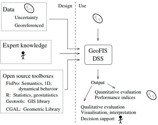
In the proposed GeoFIS architecture, all the open-source toolboxes and libraries have been selected for their ability to handle spatial data and to incorporate expert knowledge (Figure 1). Statistical and geostatistical functions dedicated to precision agriculture data (see next subsection) are implemented in R (https://www.r-project.org). Outside these specific functions, spatial data are handled through two open-source libraries, i.e., Geotools (http://www.geotools.org) and CGAL (Computational Geometry Algorithms Library, https://www.cgal.org). Geotools is used because its Java implementation allows the design of user-friendly interfaces. CGAL was chosen for its ability to provide very efficient and reliable geometric algorithms, as its functions are developed in C++. Finally, the incorporation of expert knowledge is made possible with FisPro (https://www.fispro.org), a system that uses fuzzy sets for conceptual modeling.[30]
|
GeoFIS is available in four languages (French, English, Spanish, and Portuguese). The interface is designed with a man-machine cooperation objective. The goal is to facilitate the relationships between data, learning algorithms, and expert knowledge. Documentation, scientific papers, and video tutorials are available to better understand the implemented function and to facilitate the adoption of the GeoFIS software (https://www.geofis.org/). Notifications are made when a new version of the software is available.
Functionalities implemented in GeoFIS
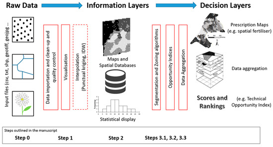
GeoFIS contains a series of low and high-level non-spatial and spatial functionalities to interrogate spatial data. The general functionalities are introduced here and then expanded in several case studies in the following section. Figure 2 shows the generic flow required in precision agriculture, from raw data processing to decision making, with the functionalities within GeoFIS at each stage indicated. In agricultural systems, data are available in different formats (points, polygons, rasters) and at different scales. The quality of the data is also variable, with some sensors being inherently noisy and others less so. Different data need potentially different approaches to (i) data validation and clean-up (quality control), (ii) data display (visualization), and, when necessary, (iii) interpolation. These steps transform data into information layers. Within GeoFIS, data can be easily imported (Step 0) and displayed as a map (in its geographical space) and as a histogram (in its attribute space). This allows the user to "expertly" identify global outliers in both the geographical and attribute space and remove any erroneous data (Step 1). Interpolation is possible using inverse distance weighting (for small data sets) and via punctual kriging with a global variogram for larger data sets (>100 points). The kriging method includes the ability to plot the experimental variogram and specify a theoretical variogram, which is then passed to the kriging function. Interpolated outputs can be directly displayed as rasters within the display (Step 2).
|
"Precision agriculture" or "smart agriculture" is only effective when effective decisions are made. End users can transform these information layers into decision layers to improve the management of their fields. Three main functionalities for management (practical) applications have been incorporated within GeoFIS to address this. Firstly, practitioners are provided with a method to delineate within-field homogeneous zones (Step 3.1). Zoning is of importance for precision agriculture data, as the identified zones will (i) facilitate spatial data visualization and interpretation and (ii) provide a spatial resolution that is practical and effective for many differential field operations. GeoFIS uses a segmentation algorithm to "zone" data layers.[18] The segmentation algorithm operates either on irregular or gridded (interpolated) data to generate potential management zones.
Secondly, while data/information collection tends to be focused around production issues, there is no restriction on its use. It can equally be used for strategic as well as tactical decision making. The example of the technical opportunity index (TOI)[31], which is implemented in GeoFIS, is a case in point. The TOI uses the production data to assess a field’s suitability for site-specific management given machinery constraints and the observed production variation (Step 3.2). The algorithm processes the within-field data with a mathematical morphological filter based on erosion and dilation.[31] This filter allows end users to account for the passes of the agricultural machinery in the field and especially the minimum area (kernel) within which it can operate reliably. As the algorithm requires the data to be organized regularly on a grid, interpolating the data might therefore be required as a pre-processing step (Step 2).
Finally, in the majority of cases, practical agronomic decisions are multi-variate in nature. Decision support therefore requires dedicated data fusion methods to merge multiple information layers into a single decision layer (Step 3.3). For instance, when available, historical yield data (high spatial resolution point information), as-applied historical fertilizer maps (polygon data), recent point soil testing (low spatial resolution point data), and early season satellite imagery (high resolution raster) should collectively feed into a decision on mid-season spatial fertilizer inputs, i.e., a prescription fertilizer map (normally a polygon layer). In the previous example, the prescription fertilization map (the decision layer) is based on a set of inputs (information layers) that are all related through expert rules. An example of a possible expert rule could be that if, on a given location in space, the observed yield is high and the soil fertilizer level is low, then it might be relevant to apply more fertilizer inputs. Within GeoFIS, the goal of the data aggregation process is to implement the expert rules so that the final spatial decision layer (that answers the question "how much fertilizer input should be applied at this particular place at this particular time?") can be obtained. Expert rules are implemented one at a time, as each rule leads to a practical agronomic decision.
Data aggregation in GeoFIS is a two-step process. First, each information layer is transformed into an expert layer, i.e., the numerical agronomic values in each information layer are transformed into degree values (from 0 to 1) according to the expert rule to be implemented. The transformation from an information layer to an expert layer is done using a fuzzy set-based function.[32] Secondly, all the expert layers are combined using an aggregation operator to respect the expert rules. Two aggregation operators are currently implemented in GeoFIS. The first operator is the Weighted Arithmetic Mean (WAM), which attributes a weight to each information source, e.g., the yield information layer may be given twice as much weight as the soil fertilizer level layer. The second operator is the Ordered Weighted Average (OWA)[33], where the weighing is slightly more complex. For a given location in space, the degree values associated with each layer involved in the expert rule are ordered, and the weights assigned to each layer will depend on their position in this ordering. This operator is of interest as it enables the implementation of logical operations, such as:
- "OR," where the expert rule applies as soon as the highest degree associated with the layers is high, and
- "AND," where the expert rule applies as soon as one of the degrees associated with the layers is high.
The result of the aggregation process is a single decision layer. The uniqueness of the GeoFIS approach is in its ability to incorporate the expert knowledge developed by farmers and advisors on the data and their fields directly into the data fusion process. The implemented data aggregation methods require the data to be collocated, either on irregular or regular grids.
Case studies
The previous section introduced the GeoFIS framework, including the functionalities implemented and how they could be adapted to the individual needs of each end user (who will have their own unique constraints on management). The following subsections provide more detailed illustrations on the main processing steps in the context of precision agriculture applications. More specifically, the three cases deal with the typical tasks that advisors and farmers may face in their daily job:
- the mapping of spatial data (Steps 0, 1 and 2),
- the evaluation and cross-comparison of the opportunity for site-specific management in their fields (Step 3.2), and
- the delineation of within-field zones for variable-rate applications where zoning is considered opportune (Steps 3.1 and 3.3).
Steps 0 to 2 will be exemplified through medium spatial resolution manual measurements performed over a banana field to map the plant vigor. High resolution yield data across several wheat fields will be used to illustrate the value of Step 3.2 to rank the fields from the most to the least suitable for site-specific management. Step 3.1 and 3.3 will be applied on a precision viticulture example aimed at defining zones for differential irrigation management. The overall objective is to demonstrate how GeoFIS has the ability to address the main issues of data processing in precision agriculture. As the three case studies are performed on different crops (banana, wheat, and grapes), each exhibiting unique characteristics, the applicability and genericity of this open-source software will also be demonstrated.
Case study 1
Rationale and description
Mapping the spatial organization in the data—An example of the vegetative response of an asynchronous plant, the banana
Variography and mapping are two very important processing steps in the precision agriculture domain. The former helps evaluate the spatial structure in the data by quantifying the proportions of (i) spatially-structured variability or large-scale variations and (ii) spatially unstructured variability or small-scale variations within the field. The latter is mainly used for the correct display of the observed spatial variability and facilitate the process of decision making.
In this case study, GeoFIS was used to investigate and map the spatial variability in the pseudostem (trunk) circumference of banana crops. The proposed analysis was carried out on this crop for two major reasons. First of all, the spatial variability in the agronomic properties of banana crops has been poorly reported in the literature.[34] Secondly, this crop is known to be asynchronous in its production cycle, which means that spatial analyses are to be handled differently from what is commonly done in annual crops, e.g., wheat, canola, or perennial ones, e.g., grapes.[34] The proposed analysis (i) estimates the proportion of spatially-structured variability in pseudostem circumferences, i.e., the proportion of variance that is mainly due to spatially-structured environmental properties[15]; (ii) determines the proportion of spatially unstructured variability that is due to non-spatially structured phenomena, e.g., the inter-plant variability, plant competition, replanting, and measurement accuracy among others; and (iii) maps the overall within-field variability of trunk circumference in the plantation.
The plot under study is situated in a commercial banana plantation in Njombe, Cameroon (WGS84: E: 4.612, N: 9.639) in its fifteenth flowering cycle. The pseudostem circumference measurements were only taken on plants where vegetative growth had ceased, i.e., plants that were either flowering or at a later phenological stage. There were 551 measurements taken using a tape measure at 1-m height and georeferenced with a trail type hand-held GPS (Table 1). The proposed analysis in GeoFIS consisted of the following steps: (i) the dataset was imported within GeoFIS (Step 0), (ii) pseudostem circumference values were filtered to ensure the quality of the dataset (Step 1), and (iii) variograms were fitted to the filtered datasets and interpolation was performed using kriging with a local neighborhood onto a 1×1 meter grid.
| |||||||||||||||||
Application in GeoFIS
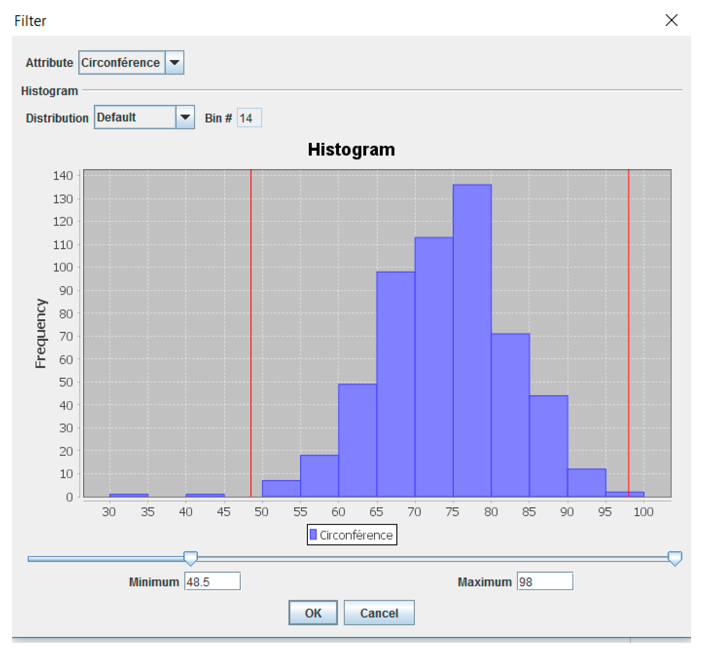
The global distribution of the data was filtered within GeoFIS (Figure 3). Users can select the attribute to be filtered at the top of the window. Below the histogram, two threshold values that represent the two tails of the distribution can be changed, by either typing specific values or moving a slide bar. Observations outside these thresholds are then removed from the dataset. Note that there were two low values in this data set that were considered outside the normal distribution by the user (Figure 3). The lower threshold allowed the user to eliminate these non-compliant values.
|
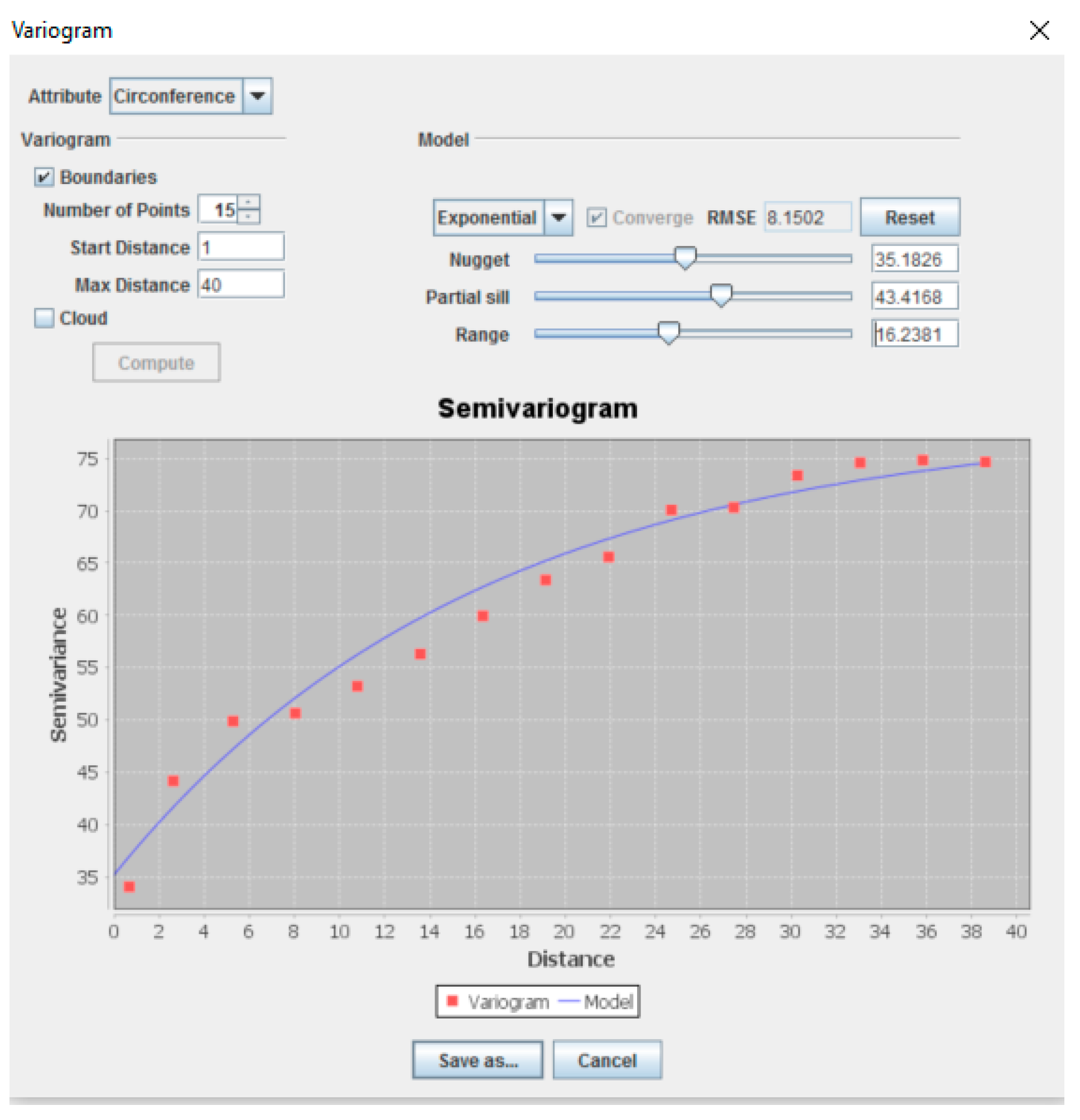
The spatial structure of the data can then be evaluated by plotting an experimental variogram, here using the within-field pseudostem circumferences. The number of lags and the maximum lag distance can be set in the left-hand corner of the window to make sure that the variogram is relevant. The interface (Figure 4) enables the user to specify and fit a theoretical variogram model to the experimental variogram. A theoretical variogram is automatically fitted, after which users can interactively change the values of the variogram parameters, i.e., nugget, partial sill, and range to improve the fit. The quality of the fit can be assessed with the root mean square error (RMSE) value that is detailed in the top right-hand corner of the interface. The theoretical model can then be saved and used later to perform interpolation by kriging.
|
Results and discussion
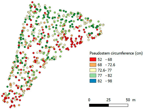
The spatial locations of the measurements are displayed in Figure 5. It clearly shows that the spatial observations are irregularly-spaced within the plot. This aspect can be simply explained by the fact that not all the banana plants had reached the flowering phenological stage (only 551 out of the 1287 plants had). In the plot under study, the pseudostem circumference exhibits a quite strong spatial autocorrelation, the ratio of autocorrelated variance being close to 55% (Table 2). This finding demonstrates that spatially-structured environmental properties, e.g., soil physical and chemical characteristics, are likely in this case to exert a relatively strong influence on the pseudostem circumference of the banana plants. The determination of the factors affecting the pseudostem circumference is beyond the scope of this study. Further analyses of, e.g., soil and plant records, might help to answer this question.
|
| ||||||||||||
Table 2 also shows that the proportion of spatially unstructured variability (C0) is not negligible. In this case study, it can be mainly explained by (i) the inherent within-plant variability that might be exacerbated by competition among neighbors, and (ii) the accuracy of the measurements which might be affected by Global Navigation Satellite Systems (GNSS) accuracy issues or operator errors.
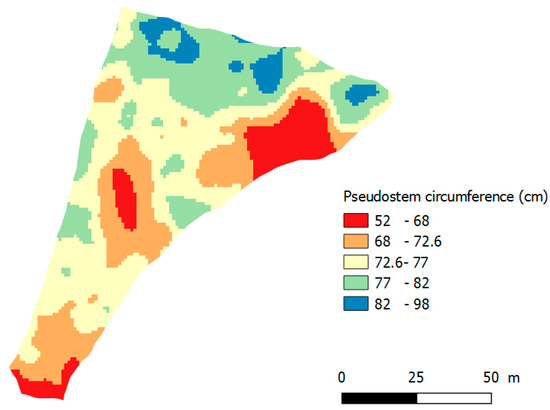
Figure 6 provides a surface (map) of the within-field pseudostem circumference after interpolation (ordinary kriging). This smooths the data in Figure 5 using information on spatial variability contained in the same data. The circumferences appear to be much lower (less than 70 cm) in the northeastern and southern portions of the plots. The larger pseudostems, those for which the circumference exceeded 87 cm, can be mainly found in the northern part of the field. Some local effects—e.g., small sites of low circumference surrounded by high pseudostem circumferences—are also visible on the maps. Those might be explained by several phenomena having a localized effect on plants, such as pest damage or replanting. It is worth recalling that this final map is not a map of circumferences of all pseudostems; rather, it's a map of potential circumference at flowering, as not all the banana plants have reached the flowering stage. This map is an alternative representation of the information displayed in Figure 5 and provides predictions for plants that were not measured in the original survey. As for Figure 6, this map may be very useful in locating sampling sites to perform further soil and/or plant analyses and to better characterize the within-field pseudostem circumference variability. It has the advantage over the raw data plot (Figure 5) of being easier for the human eye to interpret the main patterns in the field.
|
GeoFIS proved to be a relevant tool to model the spatial variability in the banana pseudostem circumference data and for continuous mapping of this property of interest. However, a couple of limitations are worth discussing. Firstly, even if the filtering interface is user-friendly, it only provides a global filtering of the data. Only the tails of the distribution can be trimmed. It may have been that spatial data exhibit not only global but also local outliers. This was not a problem here, but removing local outliers would be a useful function in the software program. When present, local outliers (inliers) will affect the quality of interpolation procedures. Secondly, GeoFIS does not yet allow the fitting of nested variogram models. This was a potential issue in this case study. In Figure 4, it could be argued that there is a short-range spatial structure within the first 10 meters and a second spatial structure from 10 to 30 meters (with a longer range). Nested spatial structures are not common but do occur in agricultural data. Thirdly, regarding the continuous mapping of the data, GeoFIS only provides a kriged map of the property of interest. The mean estimates are given, but the error (kriging variance) associated with these estimates is not provided. This is a potential limitation for assessing the mapping accuracy and for interpreting uncertainty in future analyses with the interpolated data.
Case study 2
Rationale and description
Evaluating and comparing the opportunity for site-specific management within-field
Site-specific management requires a strong investment in time, money, and technical skills for growers. This investment requires certain conditions to be met. Firstly, the within-field variability has to be strong enough to justify differentiate management. Secondly, this variability has to be spatially structured or organized enough within the field to be able to be managed by agricultural machinery.[2] Farmers, therefore, are in need of tools that will help them to evaluate this opportunity for site-specific management. To make decisions at a larger level than the field, i.e., the whole farm, this opportunity also has to be cross-compared between fields. Farmers should preferentially commit their efforts towards the fields that are the most opportune for site-specific management. These are most likely to have the largest returns on investment in agri-technology, which should minimize the risk of investment for the farmer.
In this case study, GeoFIS was used to evaluate and compare the opportunity for adopting site-specific management across multiple fields using a defined opportunity index.[31] Opportunity indices are a way of assessing if the amount and structure of variation in a field makes site-specific management a potentially feasible option.[2][25] Seven yield datasets arising from two different farms located near Evreux, in the northwestern part of France (Farm 1—WGS84: E: 0.779, N: 48.955; Farm 2—WGS84: E: 1.032, N: 48.828) were used. Fields were cropped in wheat and harvested with various combines, primarily New Holland (Turin, Italy) and Claas (Harsewinkel, Germany) combines. Yield datasets are considered particularly relevant for this case study because the yield is directly related to the field economic returns. Quantifying the amount and structure of yield variance should therefore be a valuable indicator of whether site-specific management is opportune. Structured spatial variation in yield would indicate a potential for structured spatial crop management, particularly fertilizer and agrichemicals.
This case study also demonstrates the use of GeoFIS with dense sensor-derived spatial observations, in contrast to the spatial manual measurements presented in the first case study. Yield data are collected with on-board sensors at 1 Hz as the combine traverses the field. These observations are therefore irregularly-distributed in space because (i) the intra-row and inter-row distances are different and (ii) the acquisition conditions, such as the GNSS accuracy or variable combine speed, can impact the spatial distribution of the observations. The yield information is very dense (thousands of points per hectare) and very noisy because of stochastic error in sensor operation, the intrinsic local variability in production, and errors associated with the combine harvester passing through the field.[13][28]
These seven fields were selected because they exhibit various degrees of yield autocorrelation within the same systems (farms) and, as such, should represent a different opportunity for variable-rate applications. Within this case study, several functions of GeoFIS were used to arrive at a solution that ranks and compares the seven fields in terms of a technical opportunity for site-specific management. More specifically, (i) global outliers were filtered out (Step 1); (ii) variograms were fitted to the previously filtered yield datasets, and ordinary kriging with a global variogram and local neighborhood was performed onto a 3×3 meter grid (Step 2); and (iii) the TOI was computed (see Section 2.3 Functionalities implemented in GeoFIS) (Step 3.2). To account for technical and operational constraints during the TOI computation, the following operational characteristics were assumed: a working width of 20 meters, a mean speed of three meters per second, and a delay rate of change between two different treatments of two seconds. This could be for instance the characteristics of a fertilizer spreader performing variate-rate application. The major yield statistics of the seven fields under consideration after data clean up are reported in Table 3.
| |||||||||||||||||||||||||||||||||||||||||||||
Application in GeoFIS
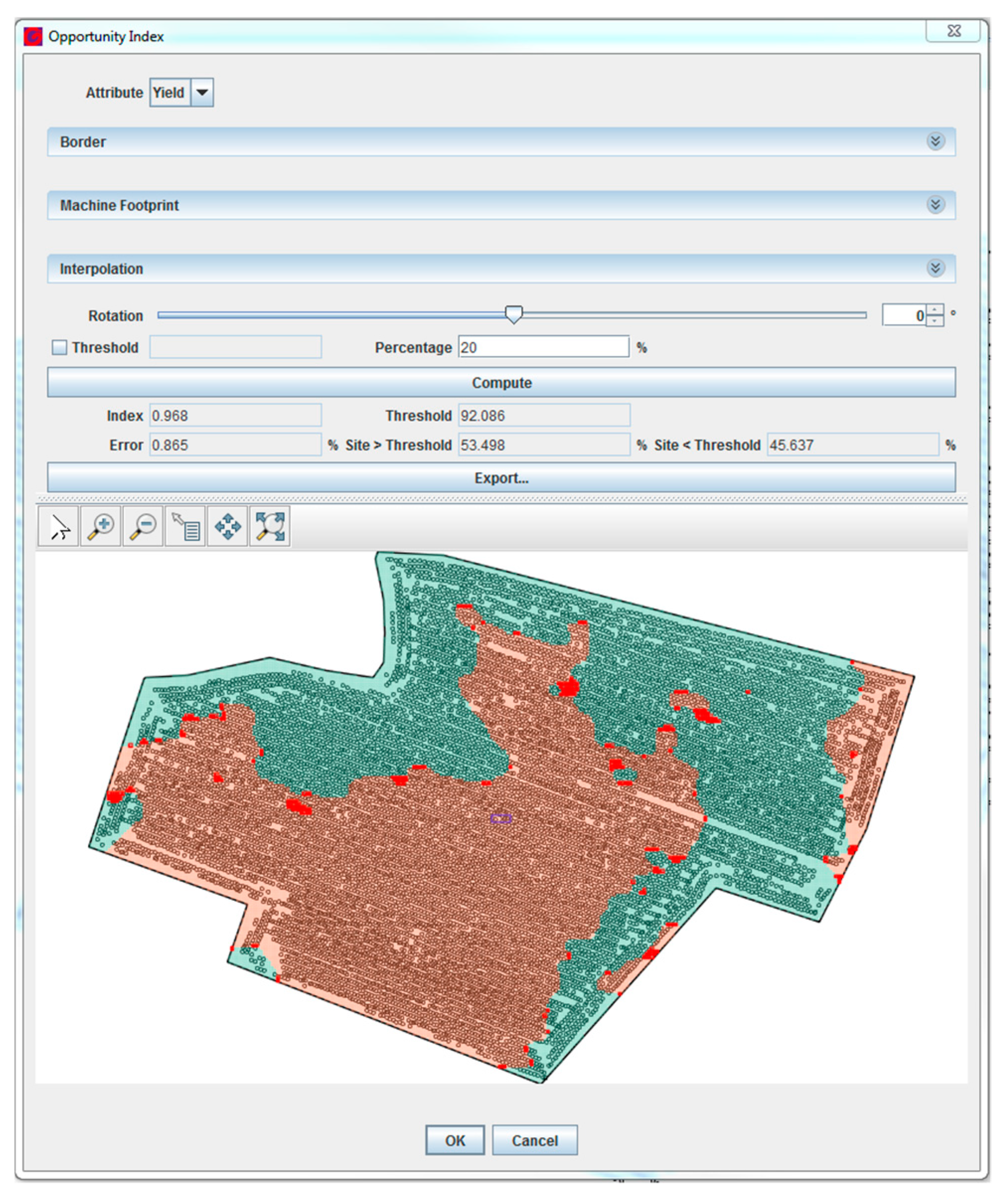
The filtering and interpolation procedures have already been detailed in the first case study and will not be discussed here. The technical opportunity index (TOI) can be computed in the Opportunity Index toolbar of the GeoFIS software. Figure 7 displays the window that appears when this menu is selected. The window is composed of three main sections. In the top drop-down menu (Border), users are asked to select the attribute on which the metric should be computed, e.g., yield, and to provide the field boundaries to make sure that the calculation of the TOI is restricted to the field of interest. Note that the boundary can be automatically derived with a convex hull; however, this may not be a good option for fields with an irregular geometric shape. In the second drop-down menu (Machine Footprint) the technical and operational constraints of future site-specific management can be specified. More specifically, users can provide the working width of machinery, its speed, the delay in the rate of change between two levels of outputs (management strategies), and the uncertainty in the GNSS positioning of the machine. The third drop-down menu (Interpolation) ensures that all observations are reported on a fixed grid and the TOI is calculated using the grid data. Users can select the size of the interpolation grid along with the interpolation procedure, i.e., inverse distance weighing or kriging. Note that both interpolation approaches need to be parameterized and require some user input.
|
When all this information has been specified by a user, the TOI can be calculated. The window displays two major outputs: (i) the TOI value associated with the data along with the corresponding error rate of application, and (ii) the potential management zone map with the different strategies that should be applied (in the case of Figure 7, there are two strategies presented). This latter map can be exported and used in other GIS software if needed.
Results and discussion
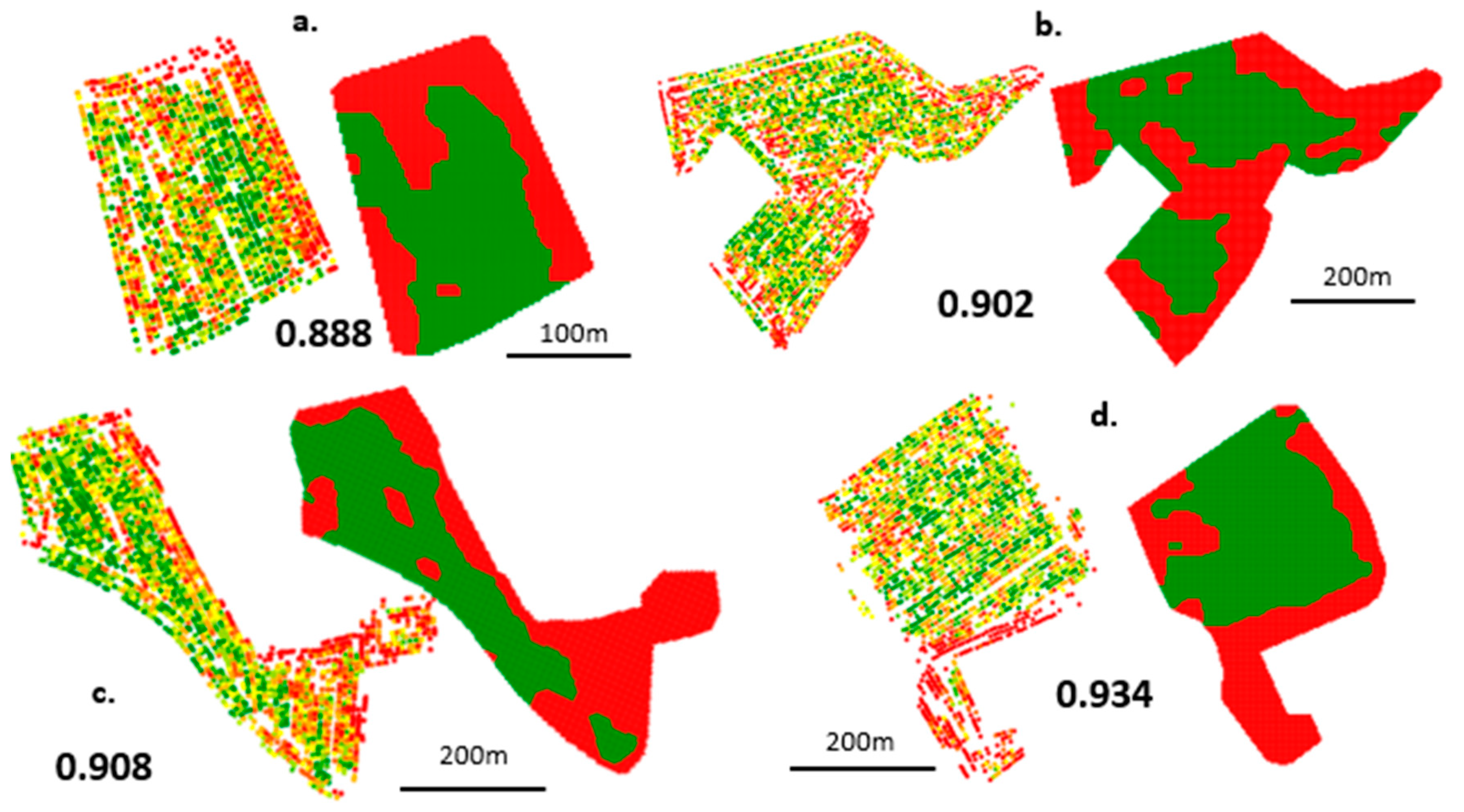
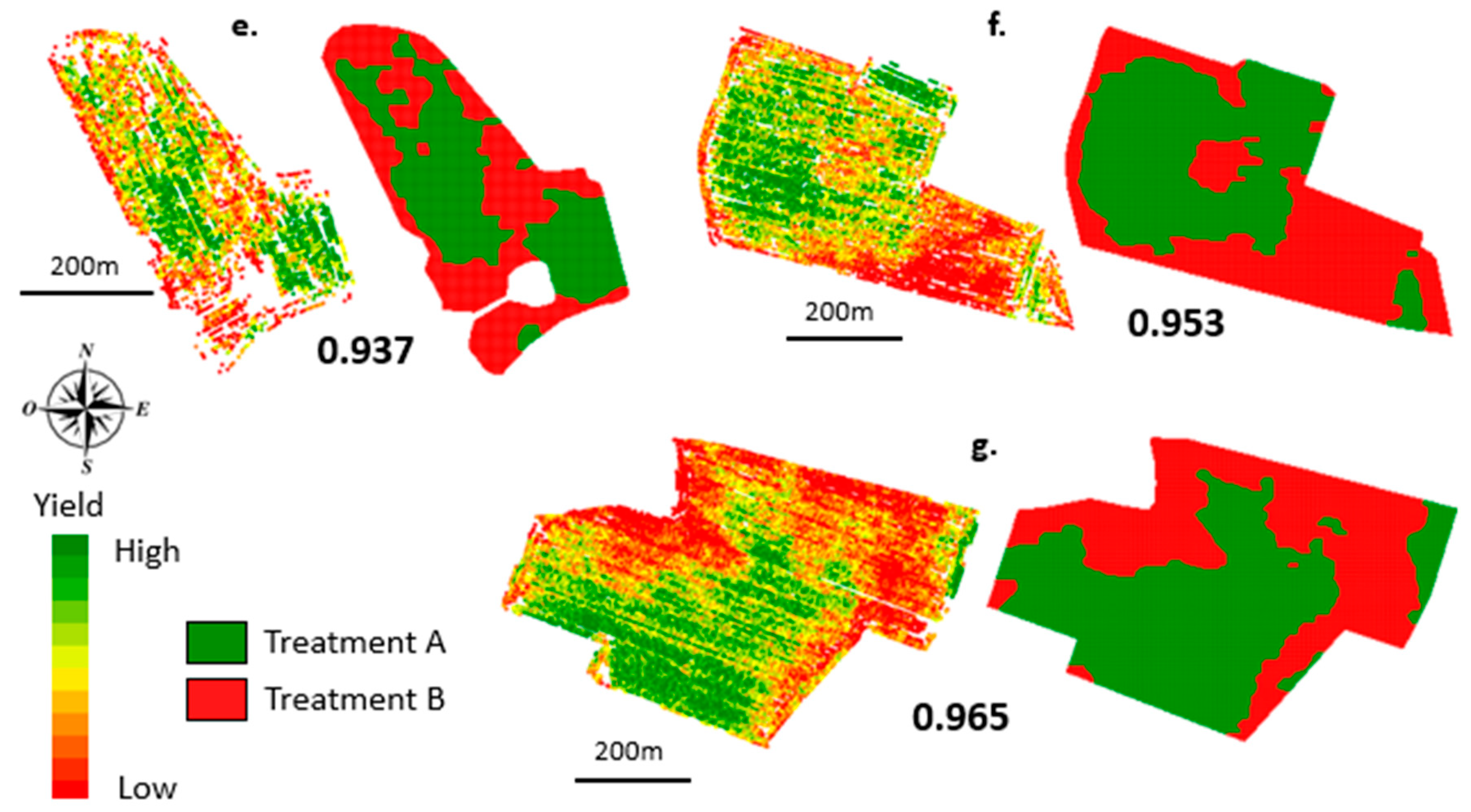
Figure 8 shows the seven fields in the study, ranked by their respective TOI values along with the corresponding variable-rate application map for a two-management strategy. It clearly shows that the fields have different levels of yield spatial structure, from the lowest for Field 1 to the strongest for Field 7. Note that, in this case study, the order of the TOI values is consistent with the order of nugget to sill ratios (Table 3). The TOI values are however very close in absolute terms (Figure 8), with a range from 0.888 to 0.965. As the TOI value can theoretically range from 0 to 1, all the fields here are exhibiting high TOI values, indicating that a site-specific management is opportune for all of these fields. All the maps have spatially-structured patterns, in accordance with the technical and operational constraints of a future possible machine pass (Figure 8). These maps could be directly incorporated into a machinery system to perform site-specific management.
|
The high TOI values for these fields is due to two principal reasons: (i) the data interpolation and (ii) the operational constraints that were set. The computation of the TOI requires the data to be regularly distributed over the field, which is why a prior interpolation procedure is put into place. In this case study, the interpolation by kriging generated a relatively strong data smoothing that artificially increased the TOI values, as it is calculated on the interpolated data. Indeed, as the small-scale variations are smoothed, the yield patterns appear much more organized in space, and the site-specific management is consequently considered more opportune. The settings of the operational characteristics in these fields also facilitated high TOI values. As the minimal size of field management (working width of the machinery) decreases, the opportunity for variable-rate application will increase. Smaller machinery means that smaller areas of spatial variation become potentially manageable. In contrast, if field management were done at a coarser level, e.g., the working width of the machinery was set to 40 meters, then the opportunity for site-specific management would decrease, and there would likely be larger differences among the seven studied fields (data not shown). As can be seen in Figure 8, only two management strategies are proposed for each field. Even if this two-class categorization appears sufficient in some case studies, the actual computation of the TOI at the moment does not allow for alternative management strategies (three, four, …, etc. classes) to be simultaneously considered. This aspect will be investigated in further studies.
The TOI is a valuable metric to evaluate and rank fields with respect to the opportunity for site-specific management. GeoFIS is an interesting tool to perform this case study because all the steps required to compute the TOI can be performed within the program. Note that potential management zone maps are also provided and can be simply exported through the easy-to-use interface (however, the target rates are not yet determined at this point; see the next case study). This should foster the adoption of precision agriculture technologies. Users must however be cautious when computing and interpreting the TOI, as this metric is particularly sensitive to the interpolation of the cleaned data and the setting of the technical and operation constraints for site-specific management. Users should be able to perform a series of tests within GeoFIS to evaluate the impact of their parametrization on the TOI values and management zone maps. To cross-compare this opportunity for potential differentiate application amongst fields, authors strongly advocate the application of the exact same process with similar settings for the calculation of the final TOI metric.
Case study 3
Rationale and description
Delineating within-field zones for variable-rate applications using expert knowledge
The delineation of within-field zones is an important procedure in precision agriculture studies because it enables, or at least facilitates, growers to perform variable-rate applications. The creation of these zones is a complex process for multiple reasons: (i) there is a need to account for spatial relationships in the data, (ii) very often multiple layers of spatial information must be combined, and (iii) the decision rules associated with agronomic applications are complex and require the grower’s knowledge to be involved in the processing. In this case study, GeoFIS is used to delineate within-field zones prior to the management of irrigation and fertilization in a Spanish vineyard using several layers of information and incorporating expert knowledge. This case study is an extension of previous work by Santesteban et al.[35] Interested readers are referred to this document for more information.
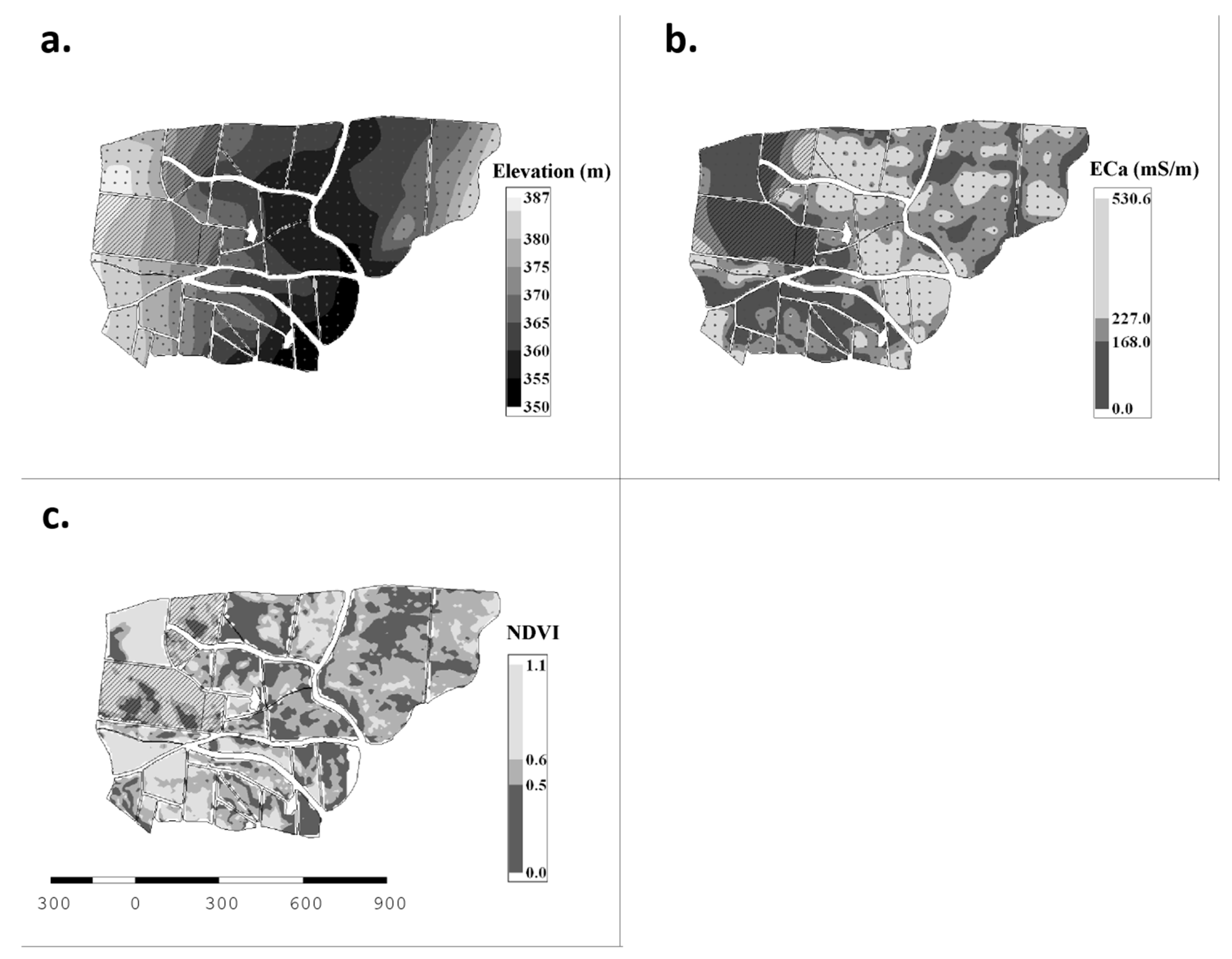
The study was carried out on a 90 hectare commercial vineyard containing 27 contiguous fields (Figure 9) located in Southern Navarre, Spain (WGS84: E: 1.405, N: 42.254). The vine vigor, soil, and water availability in the field were considered to be of major interest by the vine manager to manage irrigation and fertilization practices.
|
Grapevine vigor was estimated using the normalized difference vegetation index (NDVI) on a 3×3 meter raster layer derived from a Multi-spectral Airborne image acquired in August 2007 and provided and processed by the Geosys-Spain Company (Leica ADS40 sensor). Measurements of soil apparent electrical conductivity (ECa) on a 30×30 meter grid (256 sampling points) were performed using a handheld ground conductivity meter (EM38, Geonics Ltd., Mississauga, ON, Canada) to map soil spatial variability. The same sample sites were used to create a digital terrain model from elevation data obtained with a laser Tachymeter (TPS 1001, Leica, Heerbrugg, Switzerland). Both ECa and elevation data were kriged onto a three-meter grid. Additional monitoring was performed to provide more information on the vine vigor, soil, and water variation.[35] As these additional observations were more expensive and/or cumbersome to collect, only 64 out of the 256 sampling sites were monitored. These monitoring sites were selected using the high-resolution data layers. Additional observations were related to the (i) soil, e.g., observation of soil pits; (ii) plant, e.g., plant water status, pruning weight of wood, and yield; and (iii) production, e.g., berry size, berry composition, and yield characteristics. The analysis of all these data layers led to an explanatory reasoning summarized as[35]:
- Hydromorphic soils and wetlands are well defined by the ECa information. Their presence is mainly explained by variations in elevation.
- Vine vegetative expression is too high (and harvest quality too low) on the zones at the highest elevations, characterized by light and deep soils (low ECa values).
- Vine vegetative expression is too weak on the zones at the lowest elevations, characterized by clay soils, which suffer from water logging after rainfall events (high ECa values).
Based on this explanatory reasoning, the vineyard manager defined several decision rules to identify the situations in which the current management practices were sub-optimal regarding grape quality and quantity at harvest. An example of one of these rules was: If NDVI is high (>70) and ECa is low (<180 mS m−1) and elevation is high (>360 m), then the risk of having sub-optimal management practices is high.
This latter rule was modelled in GeoFIS to provide a map showing the risk of having sub-optimal management practices within the vineyard. First, the three data layers involved in the expert rule were transformed into risk maps using risk functions (Step 3.3). The parametrization of these risk functions was done with the vineyard manager. All the univariate risk maps were then combined into a final risk map using the OWA aggregator, which was again parameterized with the vineyard manager (see Section 2.3 Functionalities implemented in GeoFIS) (Step 3.3). Finally, a segmentation algorithm was applied to this last risk map to provide within-field risk zones (Step 3.1).
Application in GeoFIS
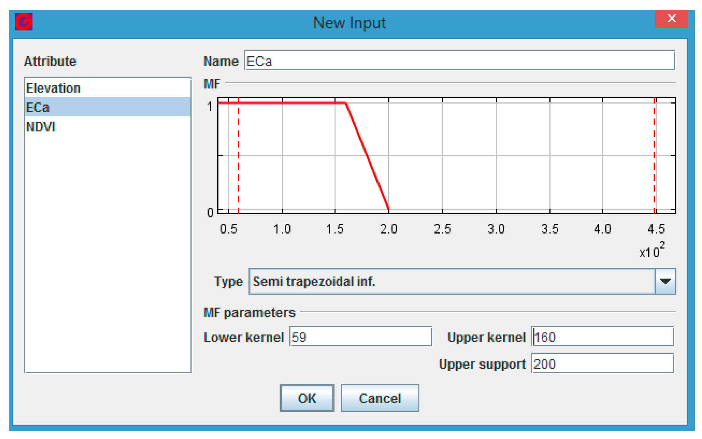
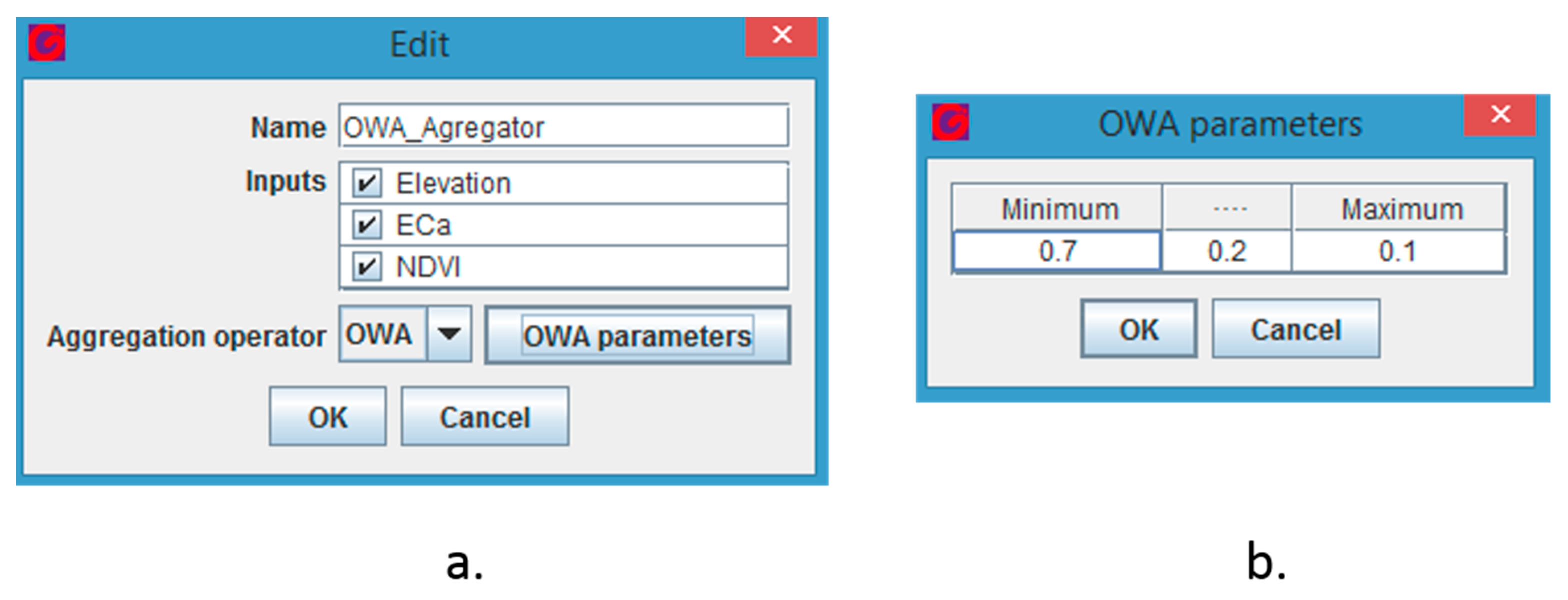
Focusing on the computation of the risk functions and on the zoning of the resulting risk map, for each layer of information (ECa, NDVI, Elevation), risk functions can be defined within GeoFIS by implementing fuzzy rules as displayed in Figure 10. Here, a semi-trapezoidal function was used to model the risk of having sub-optimal practices by solely relying on the ECa layer. In this interface, the form of the risk function can be changed along with the associated fuzzy parameters, i.e., the kernel and support. Once the risk functions have been set for all the layers of interest, all the risks can be aggregated with respect to the aforementioned expert rule(s). This aggregation procedure can be performed through the interfaces displayed in Figure 11 where (i) the layers can be selected and the aggregation operator can be chosen (OWA aggregator here) and, (ii) the parameters associated to the OWA aggregator can be stated.
|
|
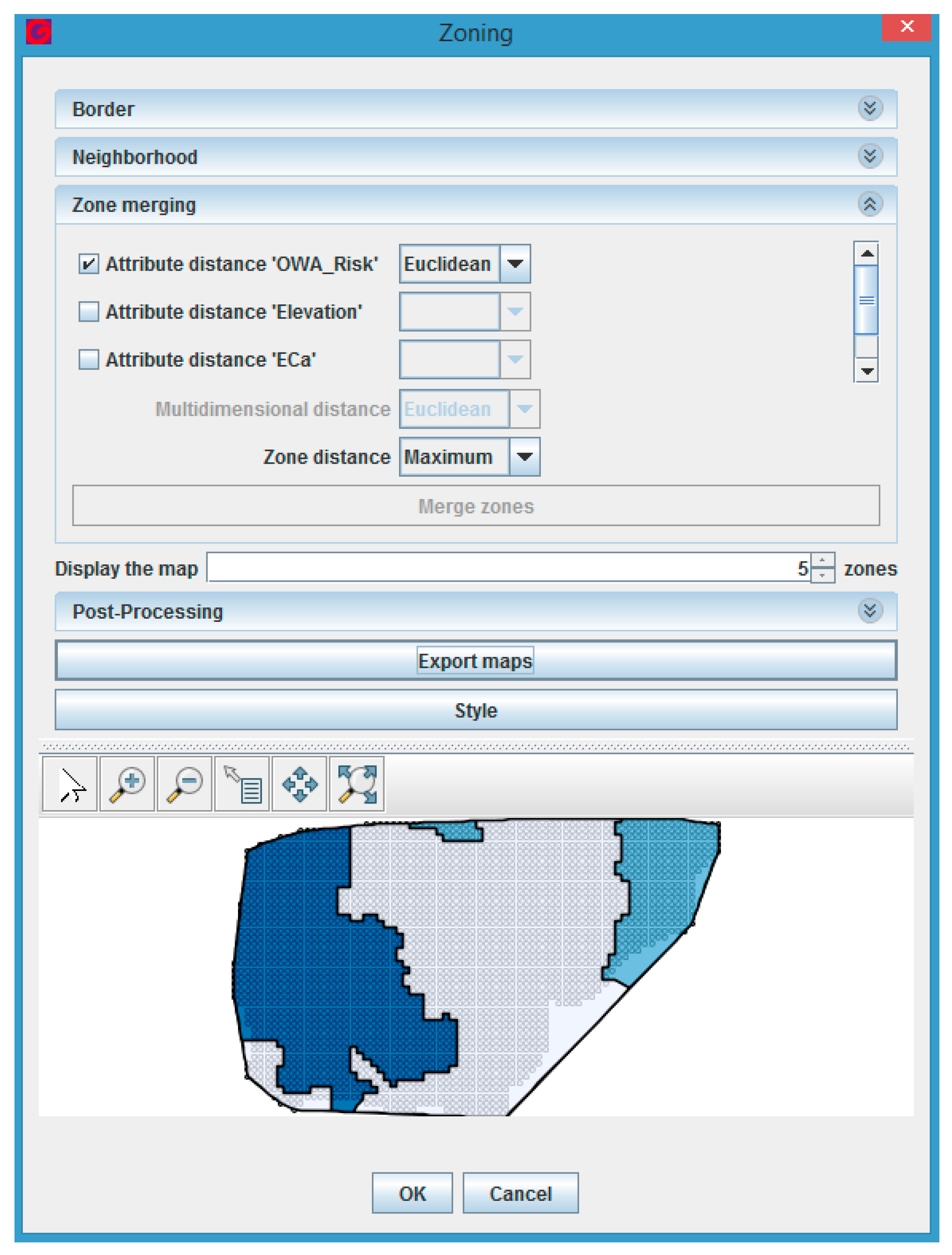
After the aggregation procedure has been run, practitioners end up with a continuous map of the global risk of having sub-optimal practices within the vineyard. To facilitate the interpretation of the map and the process of decision-making, the risk map can be zoned using the interface displayed in Figure 12. Before zoning, users must (i) define the boundary of the map, either by importing a predefined boundary or by using a default convex hull algorithm (that is proposed in GeoFIS) to generate a boundary and (ii) set the neighborhood associated to each spatial observation so that zones can be expanded using spatial neighbors. The zoning procedure can then be applied to the OWA risk map using the zoning algorithm implemented in GeoFIS.[18] Users can then display a risk map with a number of zones that they consider relevant.
|
Results and discussion
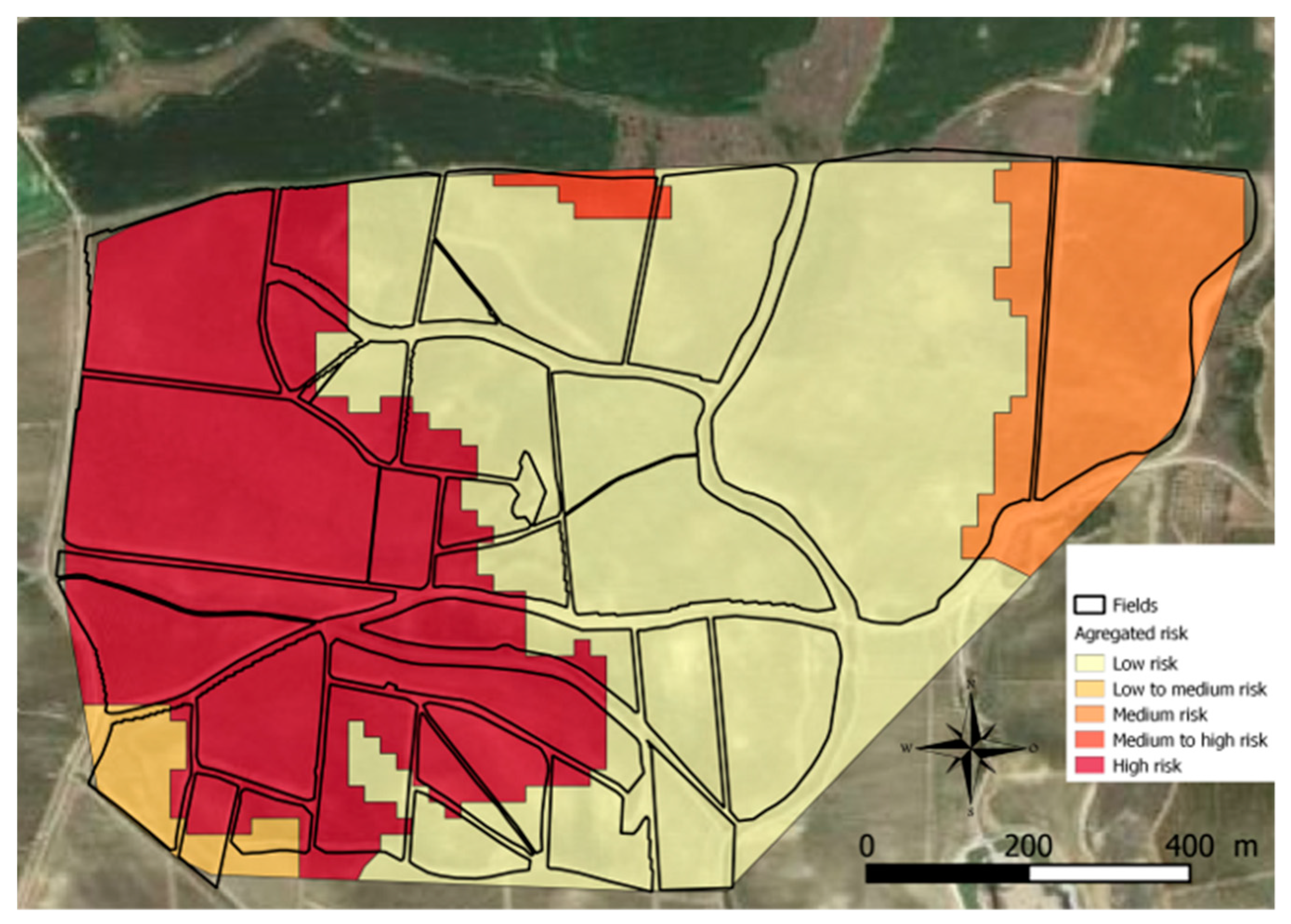
The map of the risk of arriving at sub-optimal management practices using a combination of available information and expert rules derived from local knowledge is displayed in Figure 13. This map shows five zones, three of which are relatively large, with specific risk levels. The highest risk area (dark red) is located on the western part of the vineyard and characterized by low ECa, high NDVI, and high elevation (Figure 13). In this part of the vineyard, it is likely that current management practices are not well adapted. Grape quality and quantity at harvest are not optimized in this area, and “nitrogen applications should be avoided; water availability should be reduced by the introduction of a cover crop; and Regulated Deficit Irrigation strategies should held in order to moderate shoot growth and fertility.”[35] In order to simplify the presentation of this example, only one rule has been taken into account. It would have been possible to introduce additional rules based on the work presented by Santesteban et al.[35]
|
It is interesting to note that the aggregation procedure though the OWA operator using the NDVI, ECa, and elevation layers (Figure 13) has resulted in a risk map that is different from that which would have been obtained by interpreting each layer of information independently (Figure 14). For instance, if the ECa layer had only been used to generate the risk map, the highest-risk area would have covered a much larger area of the vineyard.
|
This case study illustrates that the expertise of farm managers and advisors can be incorporated into a data-fusing algorithm to generate decision layers. Indeed, GeoFIS enables users to incorporate their own expertise, i.e., though the use of univariate risk functions/fuzzy rules, into the generation of risk maps. The use of fuzzy rules to account for this expertise is of interest as it makes it possible to avoid abrupt changes in risk and generates a more gradual variation in potential risk (Figure 10). The GeoFIS interface enables users to calibrate the risk and aggregation functions empirically by offering users the ability to test a calibration, visualize the resulting risk maps, and possibly adjust it to their convenience. However, it must be stated that this will require farmers and advisors to be supported so that their expertise can be translated correctly into the data aggregation algorithms.
The calibration of the OWA index presented in this case study (weight of 0.7 for the minimum value of univariate risk, 0.2 for the median value, and 0.1 for the maximum value) resulted from an iterative calibration process lead by the vineyard manager. This aggregation setting has strong similarities with the logical operation “AND,” i.e., the resulting risk is high if the minimum value of univariate risk is also high because it has the strongest weight. In other words, all the univariate risks are high because the median and maximum values for a univariate risk are necessarily higher than the minimum value of the univariate risk. Note that the real logical operation “AND” would be reproduced by changing the set of weights (1;0;0). By changing these weights, practitioners might also be able to reproduce the logical operation “OR” (0;0;1) for which the resulting risk is high as soon as the maximum value of a univariate risk is high. It would also be possible to perform a simple average of the different univariate risks by using the same weights for each layer.
From a more general perspective, GeoFIS simplifies the processing of the three layers of information, as the entire process was done within a single software platform. It can be compared to the data processing by Santesteban et al.[35] in which data where cleaned with Excel, interpolated with Vesper, analyzed with Matlab, and represented with ArcGIS.
Conclusions
The increasing flow of precision agriculture data requires the development of free and open-source processing software to manage and make use of these data and promote precision agriculture adoption. As such, GeoFIS has been specifically designed to facilitate the movement from spatial data to spatial information and to spatial decision making. The application of GeoFIS on some example case studies that agricultural professionals may face when dealing with spatial data has demonstrated the potential of this software. GeoFIS is a released product; however, it is important to state that all the functionality currently introduced and implemented in GeoFIS are still areas of active investigation by the scientific community. GeoFIS will be updated when, and if, improved methodologies become available. It is one of the strengths of the GeoFIS platform that it is able to integrate the latest research developments to make sure that users are provided with the most up-to-date, reliable, and powerful processing algorithms.
As it is, GeoFIS is an excellent tool to promote teaching in precision agriculture. Indeed, GeoFIS has already been used within many higher education institutions in France to teach researchers and professionals how to process spatial data. The user-friendly interface effectively facilitates the understanding of some major precision agriculture concepts.
The analysis of the three case studies has been an opportunity to also evaluate the limits of the current algorithms and to propose areas for future development within the software. For instance, the data filtering procedure focuses solely on global outliers, while spatial datasets may contain outliers more deeply rooted within the data and sometimes referred to as spatial outliers. A second example is that the variography analysis is limited to single data layers, while cross-variography studies might be relevant to evaluate the spatial relationships between multiple layers of information. To foster the adoption of GeoFIS, the authors are more than open to collaboration and are ready to integrate relevant algorithms for processing precision agriculture data.
Another possibility to promote the processing of precision agriculture data would be to create links between GeoFIS and existing GIS programs such as QGIS, an open-source GIS already widely used by many communities working on spatial data. There is a possibility to integrate all the algorithms of GeoFIS directly within this open-source GIS software to benefit from the display and processing algorithms already implemented in QGIS. This would however require users to process their precision agriculture data in a more complex environment for which specific GIS skills are necessary. Another option is to transform GeoFIS into a web-based service, rather than its current download and desktop application structure, so that users would not have to care about the R installation, Java updates, and compatibility between different operating systems.
Acknowledgements
Author contributions
J.-L.L. and S.G. developed the GeoFIS software; B.T., J.T., O.N., H.J. and S.G. conceived and designed the experiments; J.L., C.L., and L.P. performed the experiments and analyzed the data; all the authors contributed to reagents/materials/analysis tools; C.L. organized the writing of the paper.
Funding
This research received no external funding.
Conflicts of interest
The authors declare no conflict of interest.
References
- ↑ Oliver, M.A., ed. (2010). Geostatistical Applications for Precision Agriculture. Springer. pp. 331. doi:10.1007/978-90-481-9133-8. ISBN 9789048191321.
- ↑ 2.0 2.1 2.2 Pringle, M.J.; McBratney, A.B.; Whelan, B.M.; Taylor, J.M. (2003). "A preliminary approach to assessing the opportunity for site-specific crop management in a field, using yield monitor data". Agricultural Systems 76 (1): 273–92. doi:10.1016/S0308-521X(02)00005-7.
- ↑ Acevedo-Opazo, C.; Tisseyre, B.; Guillaume, S.; Ojeda, H. (2008). "The potential of high spatial resolution information to define within-vineyard zones related to vine water status". Precision Agriculture 9 (5): 285–302. doi:10.1007/s11119-008-9073-1.
- ↑ Bramley, R.G.V. (2005). "Understanding variability in winegrape production systems 2. Within vineyard variation in quality over several vintages". Australian Journal of Grape and Wine Research 11 (1): 33–42. doi:10.1111/j.1755-0238.2005.tb00277.x.
- ↑ Verdugo-Vásquez, N.; Acevedo-Opazo, C.; Valdés-Gómez, H. et al. (2016). "Spatial variability of phenology in two irrigated grapevine cultivar growing under semi-arid conditions". Precision Agriculture 17 (2): 218–45. doi:10.1007/s11119-015-9418-5.
- ↑ Baluja, J.; Diago, M.P.; Goovaerts, P.; Tardaguila, J. (2012). "Assessment of the spatial variability of anthocyanins in grapes using a fluorescence sensor: Relationships with vine vigour and yield". Precision Agriculture 13 (4): 457–72. doi:10.1007/s11119-012-9261-x.
- ↑ Debuisson, S.; Germain, C.; Garcia, O. et al. (2010). "Using Multiplex And Greenseeker To Manage Spatial Variation Of Vine Vigor In Champagne". Proceedings of the 10th International Conference on Precision Agriculture. https://www.ispag.org/proceedings/?action=abstract&id=197.
- ↑ Taylor, J.A.; Acevedo–Opazo, C.; Ojeda, H.; Tisseyre, B. (2010). "Identification and significance of sources of spatial variation in grapevine water status". Australian Journal of Grape and Wine Research 16 (1): 218–26. doi:10.1111/j.1755-0238.2009.00066.x.
- ↑ Taylor, J.A.; McBratney, A.B.; Whelan, B.M. (2007). "Establishing Management Classes for Broadacre Agricultural Production". Agronomy Journal 99 (5): 1366-76. doi:10.2134/agronj2007.0070.
- ↑ Jeong, J.S.; García-Moruno, L.; Hernández-Blanco, J. (2012). "Integrating buildings into a rural landscape using a multi-criteria spatial decision analysis in GIS-enabled web environment". Biosystems Engineering 112 (2): 82–92. doi:10.1016/j.biosystemseng.2012.03.002.
- ↑ Yalew, S.G.; van Griensven, A.; van der Zaag, P. (2016). "AgriSuit: A web-based GIS-MCDA framework for agricultural land suitability assessment". Computers and Electronics in Agriculture 128 (10): 1–8. doi:10.1016/j.compag.2016.08.008.
- ↑ Leroux, C.; Jones, H.; Clenet, A. et al. (2018). "A general method to filter out defective spatial observations from yield mapping datasets". Precision Agriculture: 1–20. doi:10.1007/s11119-017-9555-0.
- ↑ 13.0 13.1 13.2 Sudduth, K.A.; Drummond, S.T. (2006). "Yield Editor". Agronomy Journal 99 (6): 1471–82. doi:10.2134/agronj2006.0326.
- ↑ Hengl, T.; Heuvelink, G.B.M.; Stein, A. (2004). "A generic framework for spatial prediction of soil variables based on regression-kriging". Geoderma 120 (1–2): 75–93. doi:10.1016/j.geoderma.2003.08.018.
- ↑ 15.0 15.1 Oliver, M.A.; Webster, R. (2014). "A tutorial guide to geostatistics: Computing and modelling variograms and kriging". CATENA 113 (2): 56–69. doi:10.1016/j.catena.2013.09.006.
- ↑ Robinson, T.P.; Mettemicht, G. (2006). "Testing the performance of spatial interpolation techniques for mapping soil properties". Computers and Electronics in Agriculture 50 (2): 97–108. doi:10.1016/j.compag.2005.07.003.
- ↑ Cid-Garcia, N.M.; Albornoz, V.; Rios-Solis, Y.A.; Ortega, R. (2013). "Rectangular shape management zone delineation using integer linear programming". Computers and Electronics in Agriculture 93 (4): 1–9. doi:10.1016/j.compag.2013.01.009.
- ↑ 18.0 18.1 18.2 Pedroso, M.; Taylor, J.; Tisseyre, B. et al. (2010). "A segmentation algorithm for the delineation of agricultural management zones". Computers and Electronics in Agriculture 70 (1): 199–208. doi:10.1016/j.compag.2009.10.007.
- ↑ Blackmore, S.; Godwin, R.J.; Fountas, S. (2003). "The Analysis of Spatial and Temporal Trends in Yield Map Data over Six Years". Biosystems Engineering 84 (4): 455–66. doi:10.1016/S1537-5110(03)00038-2.
- ↑ Li, Y.; Shi, Z.; Li, F.; Li, H.-Y. (2007). "Delineation of site-specific management zones using fuzzy clustering analysis in a coastal saline land". Computers and Electronics in Agriculture 56 (2): 174–86. doi:10.1016/j.compag.2007.01.013.
- ↑ Oliver, Y.M.; Robertson, M.J.; Wong, M.T.F. (2010). "Integrating farmer knowledge, precision agriculture tools, and crop simulation modelling to evaluate management options for poor-performing patches in cropping fields". European Journal of Agronomy 32 (1): 40–50. doi:10.1016/j.eja.2009.05.002.
- ↑ Pichon, L.; Besqueut, G.; Tisseyre, B. (2017). "A systemic approach to identify relevant information provided by UAV in precision viticulture". Advances in Animal Biosciences 8 (2): 823–7. doi:10.1017/S2040470017001194.
- ↑ Schenatto, K.; de Souza, E.G.; Bazzi, C.L. et al. (2017). "Use of the farmer’s experience variable in the generation of management zones". Semina, Ciências Agrárias 38 (4): 2305–21. doi:10.5433/1679-0359.2017v38n4Supl1p2305.
- ↑ Leroux, C.; Jones, H.; Clenet, A.; Tisseyre, B. (2017). "A new approach for zoning irregularly-spaced, within-field data". Computers and Electronics in Agriculture 141 (9): 196–206. doi:10.1016/j.compag.2017.07.025.
- ↑ 25.0 25.1 Roudier, P.; Tisseyre, B.; Poilvé, H.; Roger, J.-M. (2008). "Management zone delineation using a modified watershed algorithm". Precision Agriculture 9: 233. doi:10.1007/s11119-008-9067-z.
- ↑ Whelan, B.M.; McBratney, A.B.; Minasny, B. (2001). "Vesper—Spatial prediction software for precision agriculture". ECPA 2001, Proceedings of the 3rd European Conference on Precision Agriculture: 139–44. https://www.semanticscholar.org/paper/Vesper-%E2%80%93-Spatial-Prediction-Software-for-Precision-Whelan-Mcbratney/52caaed8c82c943d760e3166e75d783c26d3dfe4.
- ↑ Sudduth, K.A.; Drummond, S.T.; Myers, D.B. (2012). "Yield Editor 2.0: Software for Automated Removal of Yield Map Errors". Proceedings of the 2012 ASABE Annual International Meeting: 1–14. http://extension.missouri.edu/sare/documents/asabeyieldeditor2012.pdf.
- ↑ 28.0 28.1 Simbahan, G.C.; Dobermann, A.; Ping, J.L. (2003). "Screening Yield Monitor Data Improves Grain Yield Maps". Agronomy Journal 96 (4): 1091–102. doi:10.2134/agronj2004.1091.
- ↑ Krishnan, P.; Sharma, R.K.; Dass, A. et al. (2016). "Web-based crop model: Web InfoCrop – Wheat to simulate the growth and yield of wheat". Computers and Electronics in Agriculture 127 (9): 324–35. doi:10.1016/j.compag.2016.06.008.
- ↑ 30.0 30.1 30.2 30.3 Guillaume, S.; Charnomordic, B.; Tisseyre, B.; Taylor, J. (2013). "Soft computing-based decision support tools for spatial data". International Journal of Computational Intelligence Systems 6 (Sup. 1): 18–33. doi:10.1080/18756891.2013.818185.
- ↑ 31.0 31.1 31.2 Tisseyre, B.; McBratney, A.B. (2008). "A technical opportunity index based on mathematical morphology for site-specific management: An application to viticulture". Precision Agriculture 9 (1–2): 101–13. doi:10.1007/s11119-008-9053-5.
- ↑ Guillaume, S.; Charnomordic, B.; Loisel, P. (2013). "Fuzzy partitions: A way to integrate expert knowledge into distance calculations". Information Sciences 245 (10): 76–95. doi:10.1016/j.ins.2012.07.045.
- ↑ Yager, R.R. (1988). "On ordered weighted averaging aggregation operators in multicriteria decisionmaking". IEEE Transactions on Systems, Man, and Cybernetics 18 (1): 183–90. doi:10.1109/21.87068.
- ↑ 34.0 34.1 Lamour, J.; Naud, O.; Lechaudel, M.; Tisseyre, B. (2017). "Mapping properties of an asynchronous crop: The example of time interval between flowering and maturity of banana". Advances in Animal Biosciences 8 (2): 481–6. doi:10.1017/S2040470017000449.
- ↑ 35.0 35.1 35.2 35.3 35.4 35.5 35.6 Santesteban, L.G.; Guillaume, S.; Royo, J.B.; Tisseyre, B. (2013). "Are precision agriculture tools and methods relevant at the whole-vineyard scale?". Precision Agriculture 14 (1): 2–17. doi:10.1007/s11119-012-9268-3.
Notes
This presentation is faithful to the original, with only a few minor changes to grammar, spelling, and presentation, including the addition of PMCID and DOI when they were missing from the original reference.
