Journal:Geochemical biodegraded oil classification using a machine learning approach
| Full article title | Geochemical biodegraded oil classification using a machine learning approach |
|---|---|
| Journal | Geosciences |
| Author(s) | Bispo-Silva, Sizenando; Ferreira de Oliveira, Cleverson J.; de Alemar Barberes, Gabriel |
| Author affiliation(s) | Centro de Pesquisas Leopoldo Américo Miguez de Mello, University of Coimbra |
| Primary contact | Email: sizenando at petrobras dot com dot br |
| Editors | Malvić, Tomislav; Martinez-Frias, Jesus |
| Year published | 2023 |
| Volume and issue | 13(11) |
| Article # | 321 |
| DOI | 10.3390/geosciences13110321 |
| ISSN | 2076-3263 |
| Distribution license | Creative Commons Attribution 4.0 International |
| Website | https://www.mdpi.com/2076-3263/13/11/321 |
| Download | https://www.mdpi.com/2076-3263/13/11/321/pdf?version=1698160370 (PDF) |
Abstract
Chromatographic oil analysis is an important step for the identification of biodegraded petroleum via peak visualization and interpretation of phenomena that explain the oil geochemistry. However, analyses of chromatogram components by geochemists are comparative, visual, and consequently slow. This article aims to improve the chromatogram analysis process performed during geochemical interpretation by proposing the use of convolutional neural networks (CNN), which are deep learning techniques widely used by big tech companies. Two hundred and twenty-one (221) chromatographic oil images from different worldwide basins (Brazil, USA, Portugal, Angola, and Venezuela) were used. The open-source software Orange Data Mining was used to process images by CNN. The CNN algorithm extracts, pixel by pixel, recurring features from the images through convolutional operations. Subsequently, the recurring features are grouped into common feature groups. The training result obtained a classification accuracy (CA) of 96.7% and an area under the receiver operating characteristic (ROC) curve (AUC) of 99.7%. In turn, the test result obtained a 97.6% CA and a 99.7% AUC. This work suggests that the processing of petroleum chromatographic images through CNN can become a new tool for the study of petroleum geochemistry since the chromatograms can be loaded, read, grouped, and classified more efficiently and quickly than the evaluations applied in classical methods.
Keywords: convolutional neural network, biodegradation, organic geochemistry, Orange Data Mining, chromatogram image
Introduction
The gas chromatography (GC) technique is widely used by the oil industry and can answer questions related to the origin of the oil and the physical and chemical conditions of production, refining, and storage.[1] Recently, the emergence of artificial intelligence (AI) techniques has opened up the data processing, grouping, and classification of complex imaged data, which by extension could also be applied to classify chromatogram components.[2]
Image data are part of the analytical routine practiced by petroleum geochemists, who use the proportion among chromatographic peaks to define the precursor geological environment and identify contamination by drilling fluid, light exhaust, mixing of oils, and even biodegradation.[3][4][5]
It is important to create a routine for labeling geochemical data in a way that facilitates its extraction and transformation into information to support companies’ decision-making. The most modern way to reach this level of management is through machine learning (ML) techniques controlled by experts in the field. In the case study of this paper, the users will quickly decide whether, in their analysis, they need to extract biodegraded oils from the data. Hence, the users will be able to download data efficiently with a low risk of noise, which will enable them to obtain more accurate information.
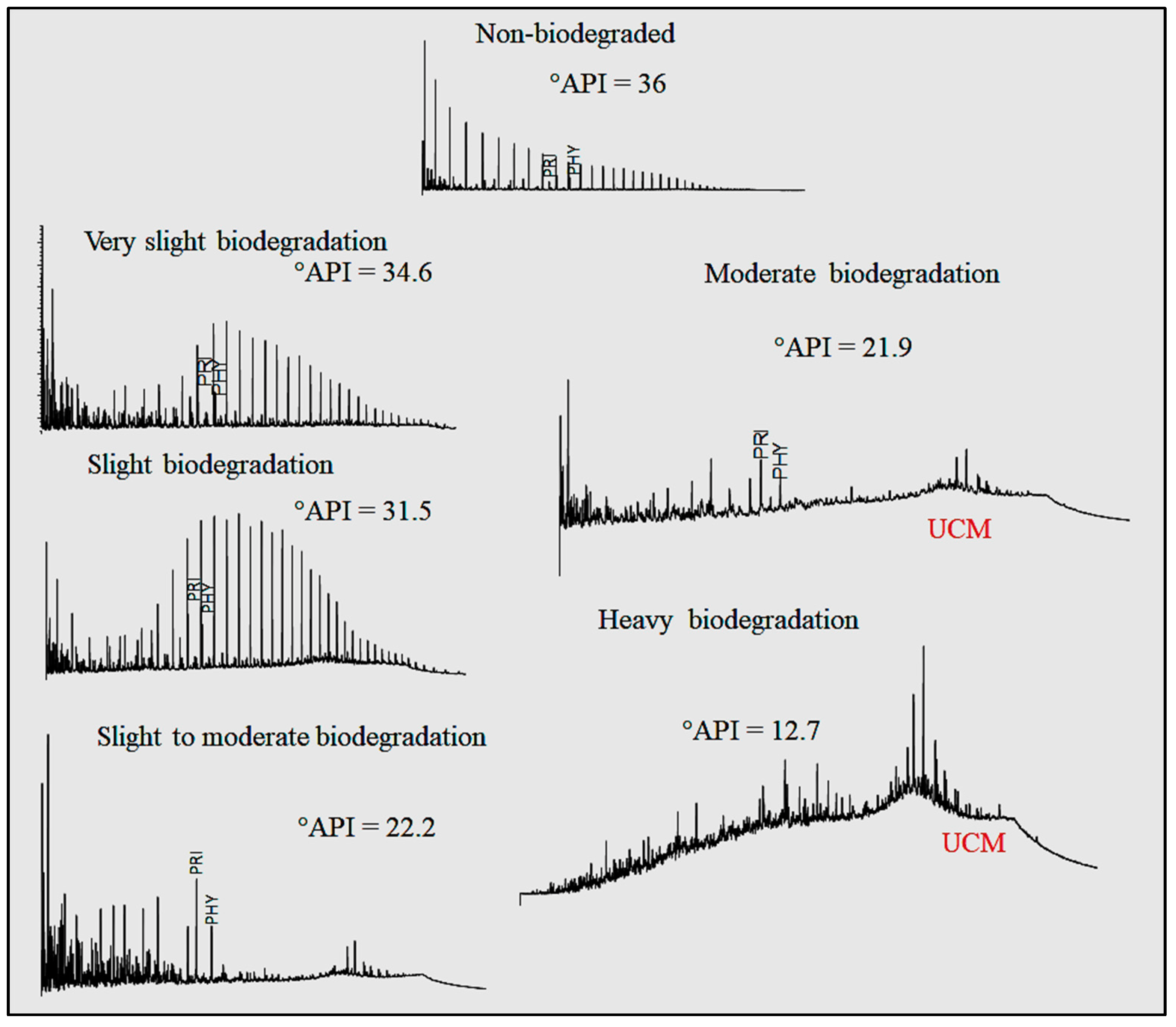
Oil biodegradation is a phenomenon caused by bacterial activity under 80 °C, often found in shallow reservoir conditions close to water/oil contact.[6][7] These bacteria tend to consume oil’s light compounds in the saturate fraction (preferably n-alkanes and then isoalkanes) and then consume aromatics. Further, there are resistant compounds that form complex chemical structures. They are located at the chromatographic baseline hump called the unresolved complex mixture (UCM).[1] As the biodegradation process is initiated, UCM tends to climb, whereas the concentration of n-alkanes decreases. These observations allowed Wenger[6] to build a biodegradation scale to rank the extent of biodegradation at five biodegradation levels: very slight, slight, moderate, heavy, and severe biodegradation (Figure 1). The biodegrading bacteria begin to consume the C8–C15 alkanes, accompanied by a very slight UCMs climb. Following, at a moderate level, bacteria consume the most part of n-alkanes (nC15+); however, UCM presents a tenuous hump.
|
The petroleum density is vital to the oil and gas industry because it implies reservoir recovery’s cost reduction together with the refined products’ quality, which can reduce production costs for companies.[5][8] The °API gravity decreases with the light compounds’ loss as well as petroleum quality.[3][6][9] This phenomenon is more sensitive at a slight to moderate biodegradation level than at a moderate to severe biodegradation level.[9]
Pristane and phytane are two iso-alkanes commonly found in petroleum and represented in petroleum chromatograms next to nC17 and nC18, respectively. The ratio between the chromatographic peaks of these compounds indicates the probable degree of biodegradation. At the level of moderate biodegradation, the pristane/phytane ratio is little changed. At a heavy level, the UCM hump is very prominent, and n-alkanes become rare.[3][6][10] When the biodegradation reaches the severe stages, biomarkers begin to be consumed, and the demethylated hopanes (25-norhopane) are formed as a result of the ring-opening process by bacteria.[10] If the reservoir underwent more than one oil’s charge and there is 25-norhopane together with n-alkanes, it suggests the oil’s pulse mixture.[3][6][8][11]
In geochemical studies of petroleum, it is common to analyze many samples or compare a few samples with previous analyses to group them, classify the characteristics of the oil, and propose a diagnosis of the studied area (e.g., well, reservoir, basin, etc.). So, in essence, the accurate evaluation of each chromatogram image can take a very long time for the geochemist due to the large number of analyses or the complexity of the samples. However, the use of AI in such geochemical analysis brings cost and time savings and reduces the possibility of interpretation errors. Despite this promise, topics related specifically to the organic geochemistry of petroleum involving the use of AI in image processing are still rare.
The use of statistics in petroleum geochemistry began around the 1960s, with simpler regression techniques and bivariate data. Subsequently, multivariate techniques with chemometrics and ML began to be used more widely because of the spread of computers and the increase in computational capacity.[12]
Chemometrics aims to explain chemical phenomena through statistical methods, which, in turn, can be processed in a computer quickly by AI algorithms (using ML and deep learning techniques). A milestone in the use of AI in petroleum geochemistry is the work of McCammon[13], who used the separation of clusters (dendrograms) in oil constituents in order to unravel which of the three horizons producers (in fields in California) would preferentially drain. Wang et al.[14] did an extensive review of the use of chemometric and ML methods in petroleum geochemistry, introducing the possibility of using concentration data in certain situations.
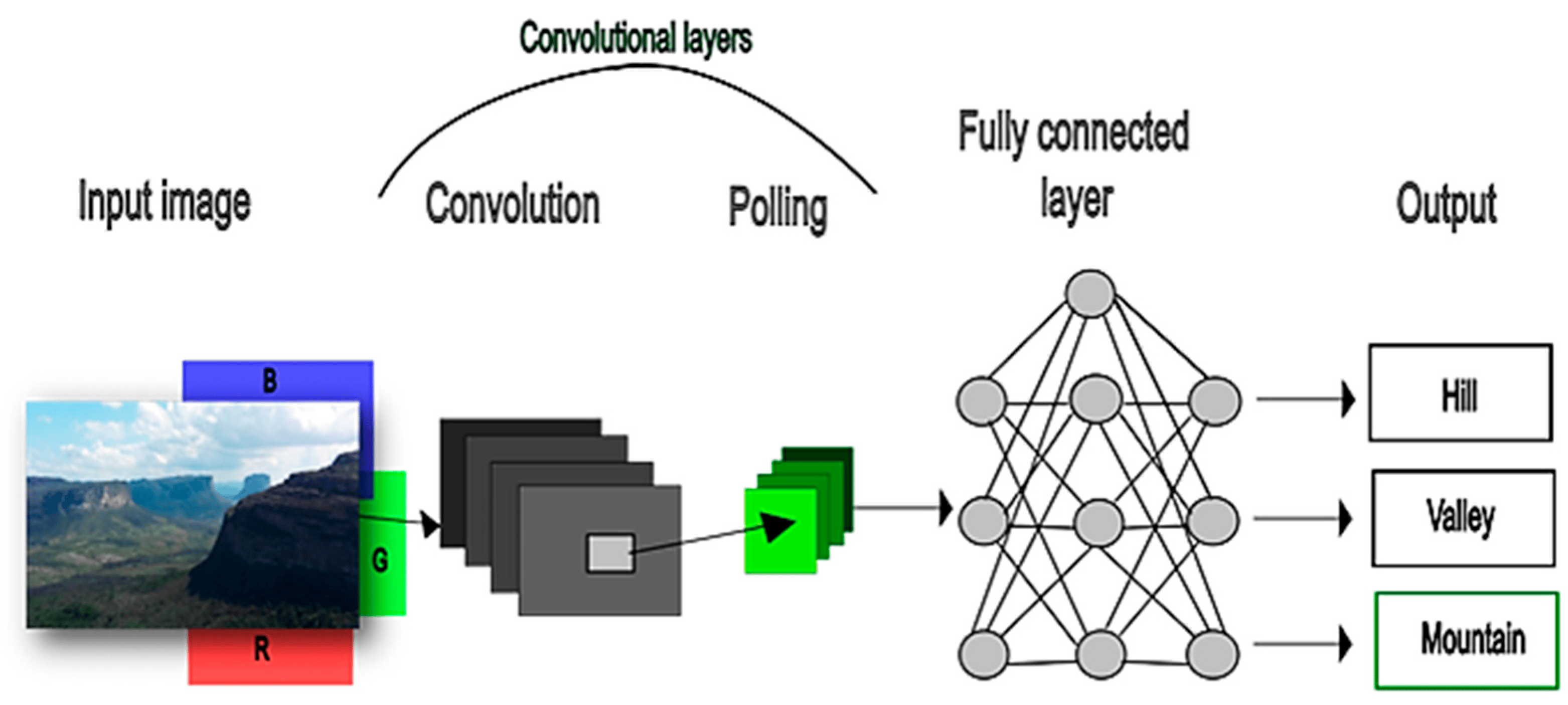
One of the main deep learning algorithms for image classification is the convolutional neural network (CNN), through which a mapping is made from images, finding recurring features and classifying them through neural networks. CNN is an algorithm used to process and classify files of the type of images that have been developed since the 1980s, but it gained popularity in 2012[15][16] when it aroused the interest of big tech. CNN is a deep learning method that caught the attention of the scientific community at the International Skin Imaging Collaboration of 2017, when the technique was used to classify images of melanomas with precision similar to experienced dermatologists, bringing speed to the diagnosis of this disease.[17][18] CNN uses a large amount of categorized image data (e.g., topographies such as hill, valley, and mountain) that are read pixel by pixel and transformed into a vector of scores, one for each category. The goal of the algorithm is that each category has the highest score, reducing the error between the output vector and the standard vector. To reduce error, the algorithm uses “weights” (millions of adjustable parameters) that control the input and output of the network and compute the vector that indicates how much a slight change in the weight could increase or decrease the mistake. This is possible because of the stochastic gradient descent (SGD), a technique responsible for presenting the input vector, calculating the output ones and their respective errors repeatedly, and readjusting the weight with each new measurement. The sum of the vector weights is computed, and when it is above a certain range, it is classified as a feature in a category.[15][19][20]
Surveys involving the use of the same or similar algorithms began to be published with topics related to other areas of knowledge. In Geology, de Lima et al.[21] used images of fossils, rock samples, cores, and petrographic samples to classify and group them, and satisfactory results were obtained. Other authors were also able to classify rock images in order to improve petrographic analysis time through ternary diagrams.[22][23] CNN has been used to classify explosive volcanic plumes[24], fossil identification[25], and unstructured geological text data clustering.[26] Koeshidayatullah et al.[27] used transfer learning[28] to classify 4,000 carbonate petrographic images in six classes, as well as nine object detection classes. Pires de Lima et al.[29] also used transfer learning to make lithofacies classifications with approximately 7,000 images split into 17 classes. These authors also compared different pre-trained models to accurately classify petrographic thin-section images.[29] CNN was successfully used to identify rock fractures from outcrop pictures and drills.[30][31] Kim et al.[32] applied CNN to identify saturation changes in core images caused by gas hydrate dissociation. With regard to source rock, the CNN coupled with an unsupervised algorithm was used in well logging data to predict total organic carbon (TOC), S2, and S1 values[33][34] and was used in seismic images to identify petroleum system elements and consequently hydrocarbon leads.[35] In addition, some papers used semantic segmentation to identify coal macerals and determine their rank.[36][37] According to some authors, CNN can be used to predict rock porosity through data logging, seismic images[38][39], and permeability.[40] Zeng and Wang[41] were able to use CNN to classify synthetic-aperture radar (SAR) images from oil spills with greater accuracy than conventional ML methods. Moreover, some authors have used CNN to classify remote-sensing image scenes.[42][43][44]
In the forensic area, Bogdal et al.[45] used chromatogram image data to classify flammable waste and determine the presence of traces of gasoline. Furthermore, in the field of organic chemistry, some works used the CNN to qualify affected peaks by elution on gas chromatography–mass spectrometry (GC-MS) chromatograms in order to discriminate the noise from the true peak.[46]
This article aims to report a process automation of image analysis with the purpose of discriminating biodegraded oils from non-biodegraded oils. The success of this test, in addition to speeding up the analysis process, brings a new look at the geochemical characterization of oils.
Materials and methods
Convolutional neural network (CNN)
The first step in using CNN was to group the image bank according to categories (continuing the example given above, hill, valley, or mountain) and load it into the algorithm. Subsequently, the data goes through a set of convolutional layers that work as an extractor of recurring features from the images, rearranging them in a feature map (Figure 2). Each neuron in the feature map of a given layer is connected with all neurons of the previous layer via weights (filter banks). Lecun et al.[15] state that all units in the feature maps share the same filter bank, mathematically corresponding to a convolution. To obtain more robust and less general features that can recognize patterns at any position in the image, a nonlinear (Kernel) calculation method is used. This step is called a "pooling layer" and is responsible for reducing the variance in feature maps with distortions or translations (Figure 2). According to Lecun et al.[15], “although the role of the convolutional layer is to detect local conjunctions of features from the previous layer, the role of the pooling layer is to merge semantically similar features into one.”
|
Soon after, each layer is stacked on top of the previous one to extract more features (fully connected layers) being extensively trained through the backpropagation mechanism and, as a result, comes out with a predicted value (category or class).
CNN using Orange
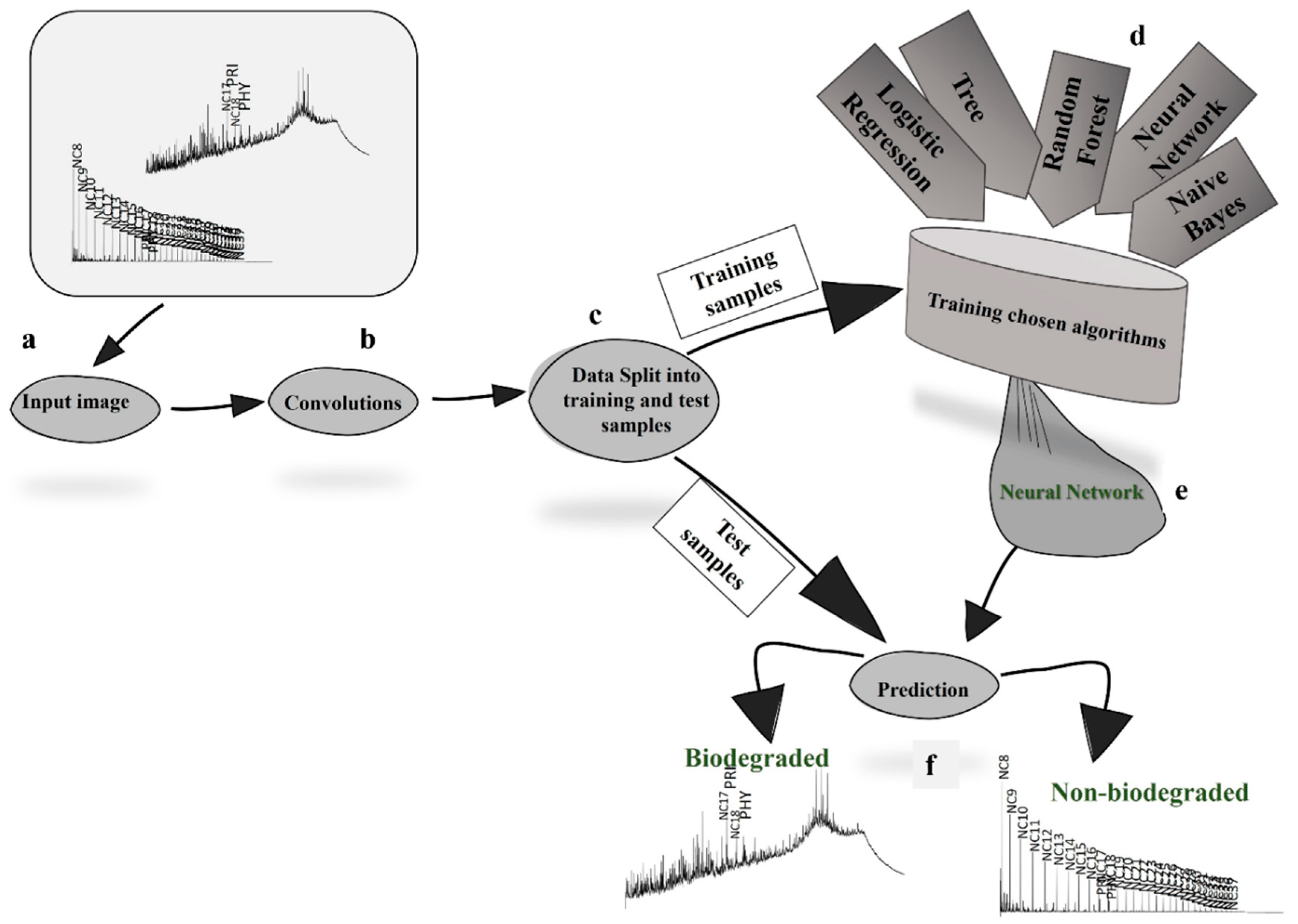
The chromatogram images were loaded into the Orange software, where the InceptionV3 CNN algorithm was used for dedication (dimension reduction or embedded) and image processing by deep learning.[47][48] InceptionV3 is a CNN model that was trained on more than one million images. However, Orange can import the inceptionV3 knowledge for training new image types (transfer learning). InceptionV3′s transfer learning is important for data with a few samples since CNN works better with larger datasets.[2][28][49][50] The deep learning processing via CNN determines the weights and feature maps of the images by finding patterns and creating filters from the training images (81% of the images). Next, ML algorithms (standard neural networks, logistic regression, decision tree, naive bayes, and random forest) were employed to classify the embedded images and compare them with each other. The algorithm with the best accuracy was utilized to generate a prediction model for the test samples (19% of the images). In the test, the model was effectively tested with untrained samples and revealed the actual efficiency of the technique for image classification. The complete flowchart of the deep learning analysis through CNN of GC-imaged data can be seen in Figure 3.
|
A total of 221 whole oil images (chromatograms) in JPEG format from GC analysis were used and tested. These data show oils from foreign basins (East Venezuela, Lusitanian, and Lower Congo, among others); however, the vast majority belong to Brazilian basins (Campos, Santos, Recôncavo, and Potiguar, among others). The samples were previously classified as both biodegraded and non-biodegraded (Figure 4 and Table 1). However, some samples were purposely misclassified as biodegraded (they are not currently biodegraded) in order to evaluate the efficiency of the classification model with mistakes still in the training stage.
|
| ||||||
The data were processed by CNN, which measured the images (180 images) and created specific filters for each category. Next, the image classifier was trained using the results calculated by the CNN to create a robust image prediction model of the chromatograms from biodegraded oils. There is a moderate difference in the number of images for each class. Nevertheless, in the test stage, the samples were stratified to avoid any bias in the model. For that, it was necessary to find the algorithm that would present the best result (accuracy).
Results
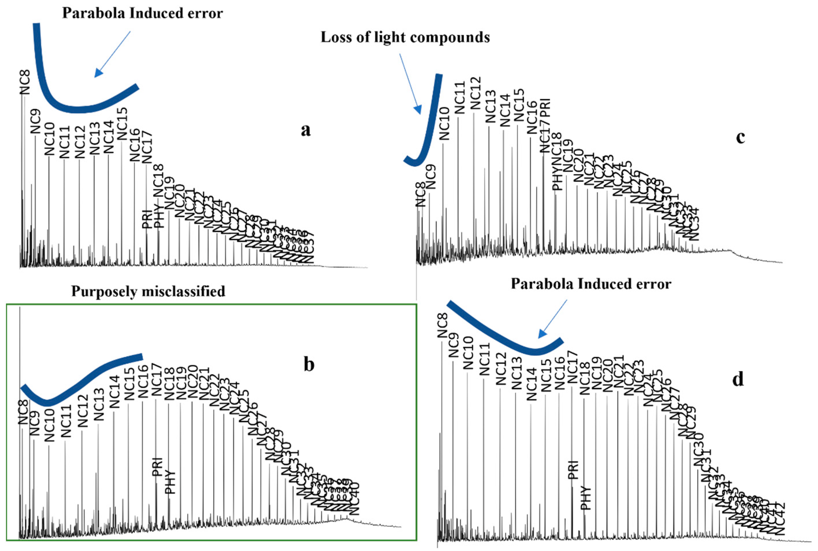
The algorithms Naive Bayes, Neural Networks, Random Forest, Decision Tree, and Logistic Regression were chosen to test the classification of images (Table 2). Neural Networks presented the best classification result because, despite having an area under the curve (AUC) as high as Logistic Regression (both with 99.7%), it presented the highest classification accuracy (CA) among all algorithms with 96.7%, followed by Logistic Regression and its 96.1%. Among the six samples that were misclassified, four show mild biodegradation with the loss of light compounds (<nC16) or a slight rise in UCM (Figure 5).
| |||||||||||||||||||||
|
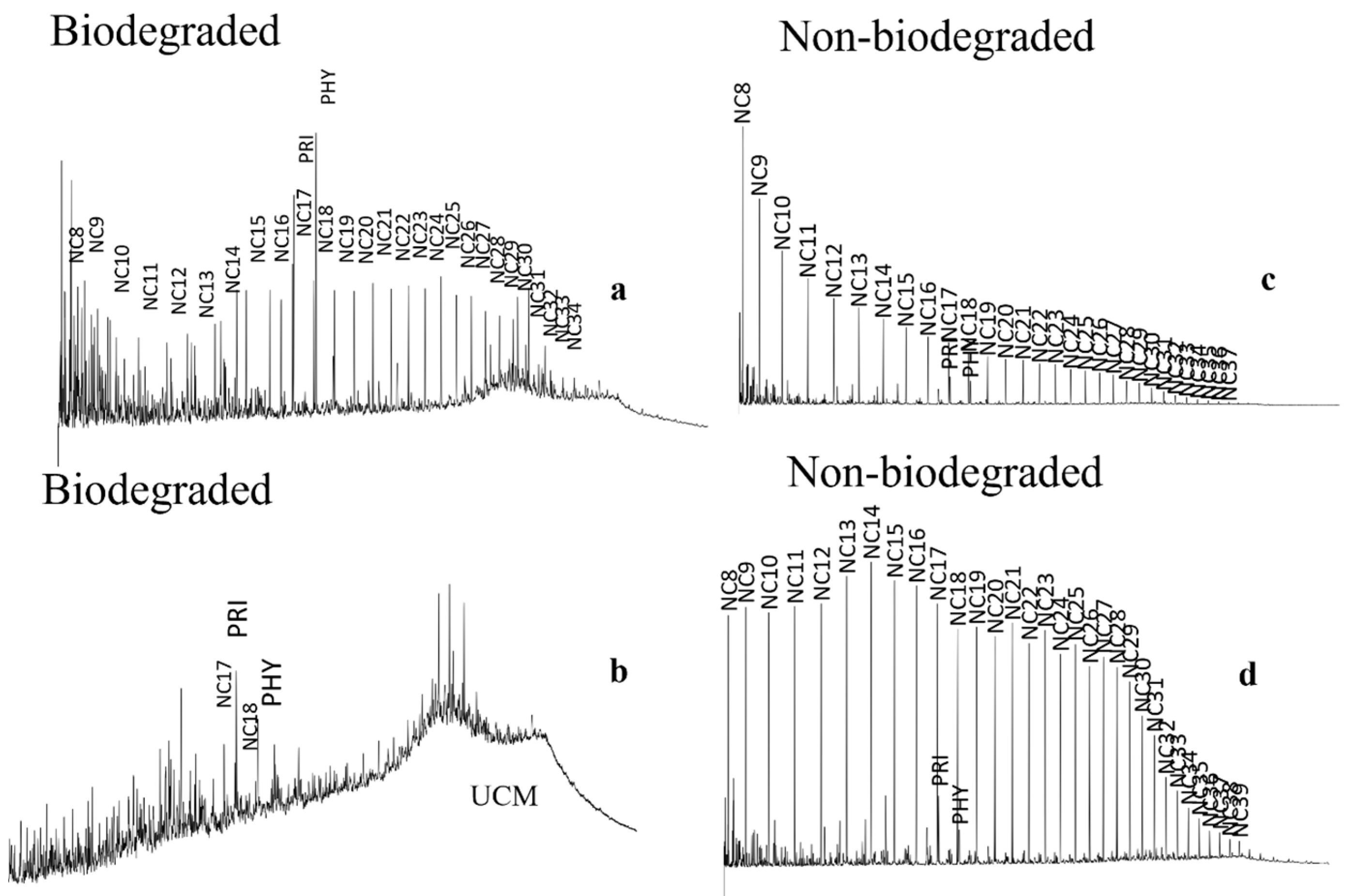
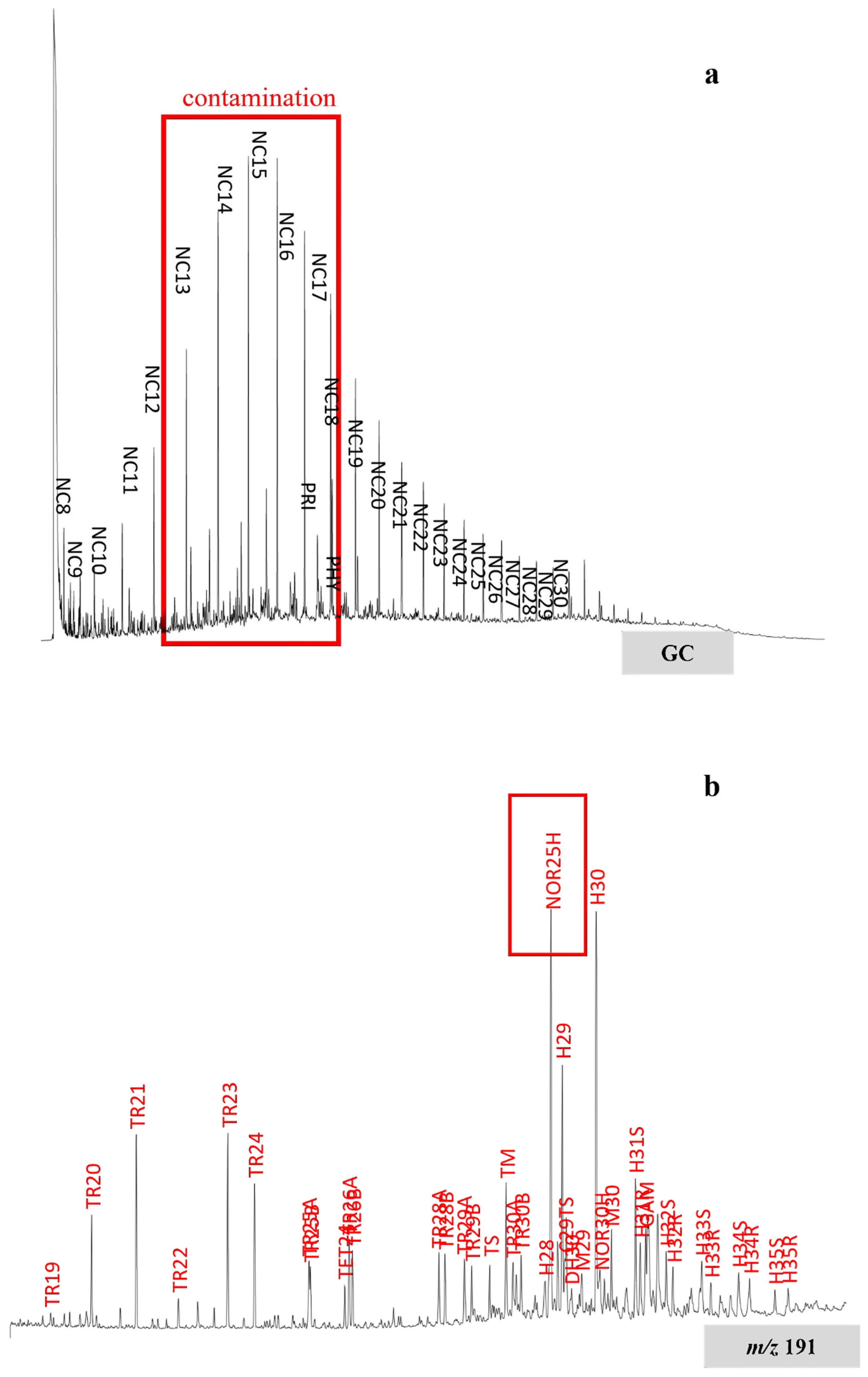
Once the prediction model was established, the next step was intended to test the model through the processing and classification of 41 images not yet classified. The test result (Table 3) shows that the AUC achieved was 99.7%, with an accuracy of 97.6%, which is even better than the training result. The confusion matrix of the test samples indicates that only one sample was misclassified; however, this sample shows characteristic elements of contamination by drilling fluid, like a prominent pike at nC13 to nC17 compounds (Figure 6a).[5] The result of the mixture of severe biodegraded oil (note the 25-norhopane peak in Figure 6b) and drilling fluid will be an oil-derived chromatogram with no distinguishable elements of biodegradation. Therefore, the test’s prediction error is actually a hit (Figure 6).
| |||||||||
|
Discussion
Samples that show only mild biodegradation features or mixtures of fluids from different sources may induce the algorithm’s prediction error (Figure 5, Figure 6, and Table 4). It is important to note that the CNN algorithm is highly dependent on the number of samples used for training. In fact, with more images, the algorithm tends to have more accurate and complex responses. Samples purposely misclassified serve as a screen for simulating cases in which the previous manual classification presents some misclassified samples. The critical point in this case study is that even small errors in the pre-classification can generate a useful and adjusted model.
| ||||||||||||||||||||||||
Some authors pointed out that it is possible to mix biodegraded oil with younger oils from fresh charges into reservoirs.[6][11] However, the better way to identify biodegraded and fresh’s mixed oils is through a m/z 177 or 191 mass chromatogram, because mass chromatograms display 25-norhopanes peaks. Nevertheless, studying mass chromatograms is beyond the scope of the present paper.
Despite the increasing use of CNN in images from rock, paleontological, and petrographic materials, the use of CNN for the improvement of organic geochemical analysis is still quite rare. Geochemists typically take eight to 16 hours to interpret 221 chromatogram images. A deep learning model can reduce this time to almost 10 minutes. Notwithstanding the success, unfortunately, CNN does not give the main parameters and details used for your interpretative mechanism.[15][21] Nevertheless, the use of CNN can open a new horizon for geochemistry when it comes to analysis by gas chromatography with flame-ionization detection (GC-FID), GC-MS, and gas chromatography with tandem mass spectrometry (GC-MS/MS) (total and selected ion chromatogram), identification of contaminants (as well as environmental pollutants), identification of analysis defects, and, finally, identification and characterization of origin and oil maturation.
Conclusions
Each well drilled for the petroleum industry increases the amount of generated oil data (e.g., isotopes, biomarkers, composition, etc.). Therefore, it is vital for these companies’ managers to manage their databases in order to simplify the download by users, who can use these geochemical data to obtain information and provide rapid support for geological modeling, well locations, and drilling resolutions.
This research proposes a new way to interpret petroleum by using a deep learning approach. The experiments were feasible to achieve high accuracy by modeling with low computational cost. This approach is sufficient to reduce the time of geochemist interpretation, and it allows companies to manage their geochemical data bank adroitly.
It is worth noting that the CNN model may also be applied to other oil classification problems such as clustering analysis, drill contamination, or even the environmental origin of parental source rock. There are possibilities for using CNN in bitumen, oil shows, or even gas samples.
Abbreviations, acronyms, and initialisms
- AI: artificial intelligence
- AUC: area under the curve
- CA: classification accuracy
- CNN: convolutional neural network
- GC: gas chromatography
- GC-FID: gas chromatography with flame-ionization detection
- GC-MS: gas chromatography–mass spectrometry
- GC-MS/MS: gas chromatography–tandem mass spectrometry
- ML: machine learning
- ROC: receiver operating characteristic
- SAR: synthetic-aperture radar
- SGD: stochastic gradient descent
- TOC: total organic carbon
- UCM: unresolved complex mixture
Acknowledgements
The authors would like to thank especially Petrobras for granting the geochemistry data used in this paper and Jarbas V. P. Guzzo for their contribution to data curation and the incentive provided.
Author contributions
S.B.-S.: Conceptualization, Methodology, Writing—Original Draft, Software manipulation. G.d.A.B.: Writing—Reviewing, and Editing; Resources. C.J.F.d.O.: Writing—Reviewing, and Editing e Data Curation. All authors have read and agreed to the published version of the manuscript.
Funding
This research received no external funding.
Data availability
Data will be made available on request.
Conflict of interest
The authors declare no conflict of interest.
References
- ↑ 1.0 1.1 Peters, Kenneth E.; Walters, C. C.; Moldowan, J. M. (2005). The biomarker guide (2nd ed ed.). Cambridge, UK ; New York: Cambridge University Press. ISBN 978-0-521-78158-9. OCLC ocm53331751. https://www.worldcat.org/title/mediawiki/oclc/ocm53331751.
- ↑ 2.0 2.1 Alzubaidi, Laith; Zhang, Jinglan; Humaidi, Amjad J.; Al-Dujaili, Ayad; Duan, Ye; Al-Shamma, Omran; Santamaría, J.; Fadhel, Mohammed A. et al. (31 March 2021). "Review of deep learning: concepts, CNN architectures, challenges, applications, future directions" (in en). Journal of Big Data 8 (1): 53. doi:10.1186/s40537-021-00444-8. ISSN 2196-1115. PMC PMC8010506. PMID 33816053. https://journalofbigdata.springeropen.com/articles/10.1186/s40537-021-00444-8.
- ↑ 3.0 3.1 3.2 3.3 Peters, Kenneth E.; Walters, C. C.; Moldowan, J. M. (2005). The biomarker guide (2nd ed ed.). Cambridge, UK ; New York: Cambridge University Press. ISBN 978-0-521-78158-9. OCLC ocm53331751. https://www.worldcat.org/title/mediawiki/oclc/ocm53331751.
- ↑ Kotarba, Maciej J.; Bilkiewicz, Elżbieta; Jurek, Krzysztof; Więcław, Dariusz; Machowski, Grzegorz (1 July 2021). "Origin, migration and secondary processes of oil and natural gas in the western part of the Polish Outer Carpathians: geochemical and geological approach" (in en). International Journal of Earth Sciences 110 (5): 1653–1679. doi:10.1007/s00531-021-02035-7. ISSN 1437-3254. https://link.springer.com/10.1007/s00531-021-02035-7.
- ↑ 5.0 5.1 5.2 Wenger, Lloyd M.; Davis, Cara L.; Evensen, Joseph M.; Gormly, James R.; Mankiewicz, Paul J. (1 November 2004). "Impact of modern deepwater drilling and testing fluids on geochemical evaluations" (in en). Organic Geochemistry 35 (11-12): 1527–1536. doi:10.1016/j.orggeochem.2004.07.001. https://linkinghub.elsevier.com/retrieve/pii/S0146638004001780.
- ↑ 6.0 6.1 6.2 6.3 6.4 6.5 Wenger, Lloyd M.; Davis, Cara L.; Isaksen, Gary H. (1 October 2002). "Multiple Controls on Petroleum Biodegradation and Impact on Oil Quality" (in en). SPE Reservoir Evaluation & Engineering 5 (05): 375–383. doi:10.2118/80168-PA. ISSN 1094-6470. https://onepetro.org/REE/article/5/05/375/109217/Multiple-Controls-on-Petroleum-Biodegradation-and.
- ↑ Röling, Wilfred F.M.; Head, Ian M.; Larter, Steve R. (1 June 2003). "The microbiology of hydrocarbon degradation in subsurface petroleum reservoirs: perspectives and prospects" (in en). Research in Microbiology 154 (5): 321–328. doi:10.1016/S0923-2508(03)00086-X. https://linkinghub.elsevier.com/retrieve/pii/S092325080300086X.
- ↑ 8.0 8.1 8.2 Wenger, Lloyd M; Isaksen, Gary H (1 December 2002). "Control of hydrocarbon seepage intensity on level of biodegradation in sea bottom sediments" (in en). Organic Geochemistry 33 (12): 1277–1292. doi:10.1016/S0146-6380(02)00116-X. https://linkinghub.elsevier.com/retrieve/pii/S014663800200116X.
- ↑ 9.0 9.1 Elias, Rouven; Vieth, Andrea; Riva, Angelo; Horsfield, Brian; Wilkes, Heinz (1 December 2007). "Improved assessment of biodegradation extent and prediction of petroleum quality" (in en). Organic Geochemistry 38 (12): 2111–2130. doi:10.1016/j.orggeochem.2007.07.004. https://linkinghub.elsevier.com/retrieve/pii/S0146638007001623.
- ↑ 10.0 10.1 Connan, Jacques (1984), "Biodegradation of Crude Oils in Reservoirs" (in en), Advances in Petroleum Geochemistry (Elsevier): 299–335, doi:10.1016/b978-0-12-032001-1.50011-0, ISBN 978-0-12-032001-1, https://linkinghub.elsevier.com/retrieve/pii/B9780120320011500110. Retrieved 2024-02-27
- ↑ 11.0 11.1 Nascimento, L.R.; Rebouças, L.M.C.; Koike, L.; de A.M Reis, F.; Soldan, A.L.; Cerqueira, J.R.; Marsaioli, A.J. (1 September 1999). "Acidic biomarkers from Albacora oils, Campos Basin, Brazil" (in en). Organic Geochemistry 30 (9): 1175–1191. doi:10.1016/S0146-6380(99)00107-2. https://linkinghub.elsevier.com/retrieve/pii/S0146638099001072.
- ↑ Hempkins, W. Brent (12 April 1978). "Multivariate Statistical Analysis In Formation Evaluation". All Days (San Francisco, California: SPE): SPE–7144–MS. doi:10.2118/7144-MS. https://onepetro.org/SPEWRM/proceedings/78CRM/All-78CRM/San%20Francisco,%20California/133959.
- ↑ McCammon, Richard B. (1968). "The Dendrograph: A New Tool for Correlation" (in en). Geological Society of America Bulletin 79 (11): 1663. doi:10.1130/0016-7606(1968)79[1663:TDANTF]2.0.CO;2. ISSN 0016-7606. https://pubs.geoscienceworld.org/gsabulletin/article/79/11/1663-1670/6295.
- ↑ Wang, Yao-Ping; Zou, Yan-Rong; Shi, Jian-Ting; Shi, Jun (1 August 2018). "Review of the chemometrics application in oil-oil and oil-source rock correlations" (in en). Journal of Natural Gas Geoscience 3 (4): 217–232. doi:10.1016/j.jnggs.2018.08.003. https://linkinghub.elsevier.com/retrieve/pii/S2468256X1830052X.
- ↑ 15.0 15.1 15.2 15.3 15.4 15.5 LeCun, Yann; Bengio, Yoshua; Hinton, Geoffrey (28 May 2015). "Deep learning" (in en). Nature 521 (7553): 436–444. doi:10.1038/nature14539. ISSN 0028-0836. https://www.nature.com/articles/nature14539.
- ↑ 16.0 16.1 Rawat, Waseem; Wang, Zenghui (1 September 2017). "Deep Convolutional Neural Networks for Image Classification: A Comprehensive Review". Neural Computation 29 (9): 2352–2449. doi:10.1162/NECO_a_00990. ISSN 1530-888X. PMID 28599112. https://pubmed.ncbi.nlm.nih.gov/28599112.
- ↑ Esteva, Andre; Kuprel, Brett; Novoa, Roberto A.; Ko, Justin; Swetter, Susan M.; Blau, Helen M.; Thrun, Sebastian (2 February 2017). "Dermatologist-level classification of skin cancer with deep neural networks" (in en). Nature 542 (7639): 115–118. doi:10.1038/nature21056. ISSN 0028-0836. PMC PMC8382232. PMID 28117445. https://www.nature.com/articles/nature21056.
- ↑ Marchetti, Michael A.; Liopyris, Konstantinos; Dusza, Stephen W.; Codella, Noel C.F.; Gutman, David A.; Helba, Brian; Kalloo, Aadi; Halpern, Allan C. et al. (1 March 2020). "Computer algorithms show potential for improving dermatologists' accuracy to diagnose cutaneous melanoma: Results of the International Skin Imaging Collaboration 2017" (in en). Journal of the American Academy of Dermatology 82 (3): 622–627. doi:10.1016/j.jaad.2019.07.016. PMC PMC7006718. PMID 31306724. https://linkinghub.elsevier.com/retrieve/pii/S0190962219323734.
- ↑ Liang, Xiaoyao (2020). Ascend AI processor architecture and programming: principles and applications of cann. Amsterdam, Netherlands: Elsevier. ISBN 978-0-12-823488-4.
- ↑ Albawi, Saad; Mohammed, Tareq Abed; Al-Zawi, Saad (1 August 2017). "Understanding of a convolutional neural network". 2017 International Conference on Engineering and Technology (ICET) (Antalya: IEEE): 1–6. doi:10.1109/ICEngTechnol.2017.8308186. ISBN 978-1-5386-1949-0. https://ieeexplore.ieee.org/document/8308186/.
- ↑ 21.0 21.1 de Lima, Rafael Pires; Bonar, Alicia; Duarte Coronado, David; Marfurt, Kurt; Nicholson, Charles (30 June 2019). Birgenheier, Lauren; Harper, Howard. eds. "Deep convolutional neural networks as a geological image classification tool". The Sedimentary Record 17 (2): 4–9. doi:10.2110/sedred.2019.2.4. https://thesedimentaryrecord.scholasticahq.com/article/31354-deep-convolutional-neural-networks-as-a-geological-image-classification-tool.
- ↑ Xu, Zhenhao; Ma, Wen; Lin, Peng; Shi, Heng; Pan, Dongdong; Liu, Tonghui (1 September 2021). "Deep learning of rock images for intelligent lithology identification" (in en). Computers & Geosciences 154: 104799. doi:10.1016/j.cageo.2021.104799. https://linkinghub.elsevier.com/retrieve/pii/S009830042100100X.
- ↑ Alférez, Germán H.; Vázquez, Elías L.; Martínez Ardila, Ana María; Clausen, Benjamin L. (1 June 2021). "Automatic classification of plutonic rocks with deep learning" (in en). Applied Computing and Geosciences 10: 100061. doi:10.1016/j.acags.2021.100061. https://linkinghub.elsevier.com/retrieve/pii/S2590197421000094.
- ↑ Wilkes, T.C.; Pering, T.D.; McGonigle, A.J.S. (1 November 2022). "Semantic segmentation of explosive volcanic plumes through deep learning" (in en). Computers & Geosciences 168: 105216. doi:10.1016/j.cageo.2022.105216. https://linkinghub.elsevier.com/retrieve/pii/S0098300422001650.
- ↑ Wang, Haizhou; Li, Chufan; Zhang, Zhifei; Kershaw, Stephen; Holmer, Lars E.; Zhang, Yang; Wei, Keyi; Liu, Peng (1 May 2022). "Fossil brachiopod identification using a new deep convolutional neural network" (in en). Gondwana Research 105: 290–298. doi:10.1016/j.gr.2021.09.011. https://linkinghub.elsevier.com/retrieve/pii/S1342937X21002665.
- ↑ Wang, Bin; Wu, Liang; Xie, Zhong; Qiu, Qinjun; Zhou, Yuan; Ma, Kai; Tao, Liufeng (1 November 2022). "Understanding geological reports based on knowledge graphs using a deep learning approach" (in en). Computers & Geosciences 168: 105229. doi:10.1016/j.cageo.2022.105229. https://linkinghub.elsevier.com/retrieve/pii/S0098300422001789.
- ↑ Koeshidayatullah, Ardiansyah; Morsilli, Michele; Lehrmann, Daniel J.; Al-Ramadan, Khalid; Payne, Jonathan L. (1 December 2020). "Fully automated carbonate petrography using deep convolutional neural networks" (in en). Marine and Petroleum Geology 122: 104687. doi:10.1016/j.marpetgeo.2020.104687. https://linkinghub.elsevier.com/retrieve/pii/S0264817220304700.
- ↑ 28.0 28.1 Bengio, Y. (2011). "Deep learning of representations for unsupervised and transfer learning". Proceedings of the 2011 International Conference on Unsupervised and Transfer Learning Workshop 27: 17–37. doi:10.5555/3045796.3045800. https://dl.acm.org/doi/10.5555/3045796.3045800.
- ↑ 29.0 29.1 Pires de Lima, Rafael; Suriamin, Fnu; Marfurt, Kurt J.; Pranter, Matthew J. (1 August 2019). "Convolutional neural networks as aid in core lithofacies classification" (in en). Interpretation 7 (3): SF27–SF40. doi:10.1190/INT-2018-0245.1. ISSN 2324-8858. https://library.seg.org/doi/10.1190/INT-2018-0245.1.
- ↑ Byun, Hoon; Kim, Jineon; Yoon, Dongyoung; Kang, Il-Seok; Song, Jae-Joon (1 December 2021). "A deep convolutional neural network for rock fracture image segmentation" (in en). Earth Science Informatics 14 (4): 1937–1951. doi:10.1007/s12145-021-00650-1. ISSN 1865-0473. https://link.springer.com/10.1007/s12145-021-00650-1.
- ↑ Alzubaidi, Fatimah; Makuluni, Patrick; Clark, Stuart R.; Lie, Jan Erik; Mostaghimi, Peyman; Armstrong, Ryan T. (1 January 2022). "Automatic fracture detection and characterization from unwrapped drill-core images using mask R–CNN" (in en). Journal of Petroleum Science and Engineering 208: 109471. doi:10.1016/j.petrol.2021.109471. https://linkinghub.elsevier.com/retrieve/pii/S0920410521011141.
- ↑ Kim, Sungil; Lee, Kyungbook; Lee, Minhui; Lee, Jaehyoung; Ahn, Taewoong; Lim, Jung-Tek (1 February 2022). "Evaluation of saturation changes during gas hydrate dissociation core experiment using deep learning with data augmentation" (in en). Journal of Petroleum Science and Engineering 209: 109820. doi:10.1016/j.petrol.2021.109820. https://linkinghub.elsevier.com/retrieve/pii/S092041052101439X.
- ↑ Wang, Huijun; Wu, Wei; Chen, Tao; Dong, Xinjun; Wang, Guangxu (1 May 2019). "An improved neural network for TOC, S1 and S2 estimation based on conventional well logs" (in en). Journal of Petroleum Science and Engineering 176: 664–678. doi:10.1016/j.petrol.2019.01.096. https://linkinghub.elsevier.com/retrieve/pii/S092041051930110X.
- ↑ Wang, Huijun; Lu, Shuangfang; Qiao, Lu; Chen, Fangwen; He, Xipeng; Gao, Yuqiao; Mei, Junwei (1 July 2022). "Unsupervised contrastive learning for few-shot TOC prediction and application" (in en). International Journal of Coal Geology 259: 104046. doi:10.1016/j.coal.2022.104046. https://linkinghub.elsevier.com/retrieve/pii/S0166516222001227.
- ↑ Souza, J.F.L.; Santos, M.D.; Magalhães, R.M.; Neto, E.M.; Oliveira, G.P.; Roque, W.L. (1 November 2019). "Automatic classification of hydrocarbon “leads” in seismic images through artificial and convolutional neural networks" (in en). Computers & Geosciences 132: 23–32. doi:10.1016/j.cageo.2019.07.002. https://linkinghub.elsevier.com/retrieve/pii/S0098300419300263.
- ↑ Lei, Meng; Rao, Zhongyu; Wang, Hongdong; Chen, Yilin; Zou, Liang; Yu, Han (1 June 2021). "Maceral groups analysis of coal based on semantic segmentation of photomicrographs via the improved U-net" (in en). Fuel 294: 120475. doi:10.1016/j.fuel.2021.120475. https://linkinghub.elsevier.com/retrieve/pii/S0016236121003513.
- ↑ Santos, Richard Bryan Magalhães; Augusto, Karen Soares; Iglesias, Julio César Álvarez; Rodrigues, Sandra; Paciornik, Sidnei; Esterle, Joan S.; Domingues, Alei Leite Alcantara (1 November 2022). "A deep learning system for collotelinite segmentation and coal reflectance determination" (in en). International Journal of Coal Geology 263: 104111. doi:10.1016/j.coal.2022.104111. https://linkinghub.elsevier.com/retrieve/pii/S0166516222001872.
- ↑ Feng, Runhai (1 May 2020). "Estimation of reservoir porosity based on seismic inversion results using deep learning methods" (in en). Journal of Natural Gas Science and Engineering 77: 103270. doi:10.1016/j.jngse.2020.103270. https://linkinghub.elsevier.com/retrieve/pii/S1875510020301244.
- ↑ Wang, Jun; Cao, Junxing; Yuan, Shan (1 December 2022). "Deep learning reservoir porosity prediction method based on a spatiotemporal convolution bi-directional long short-term memory neural network model" (in en). Geomechanics for Energy and the Environment 32: 100282. doi:10.1016/j.gete.2021.100282. https://linkinghub.elsevier.com/retrieve/pii/S2352380821000496.
- ↑ Wu, Jinlong; Yin, Xiaolong; Xiao, Heng (1 September 2018). "Seeing permeability from images: fast prediction with convolutional neural networks" (in en). Science Bulletin 63 (18): 1215–1222. doi:10.1016/j.scib.2018.08.006. https://linkinghub.elsevier.com/retrieve/pii/S2095927318303955.
- ↑ Zeng, Kan; Wang, Yixiao (22 March 2020). "A Deep Convolutional Neural Network for Oil Spill Detection from Spaceborne SAR Images" (in en). Remote Sensing 12 (6): 1015. doi:10.3390/rs12061015. ISSN 2072-4292. https://www.mdpi.com/2072-4292/12/6/1015.
- ↑ Pires de Lima, Rafael; Marfurt, Kurt (25 December 2019). "Convolutional Neural Network for Remote-Sensing Scene Classification: Transfer Learning Analysis" (in en). Remote Sensing 12 (1): 86. doi:10.3390/rs12010086. ISSN 2072-4292. https://www.mdpi.com/2072-4292/12/1/86.
- ↑ Hu, Fan; Xia, Gui-Song; Hu, Jingwen; Zhang, Liangpei (5 November 2015). "Transferring Deep Convolutional Neural Networks for the Scene Classification of High-Resolution Remote Sensing Imagery" (in en). Remote Sensing 7 (11): 14680–14707. doi:10.3390/rs71114680. ISSN 2072-4292. http://www.mdpi.com/2072-4292/7/11/14680.
- ↑ Yu, Donghang; Xu, Qing; Guo, Haitao; Zhao, Chuan; Lin, Yuzhun; Li, Daoji (2 April 2020). "An Efficient and Lightweight Convolutional Neural Network for Remote Sensing Image Scene Classification" (in en). Sensors 20 (7): 1999. doi:10.3390/s20071999. ISSN 1424-8220. PMC PMC7181261. PMID 32252483. https://www.mdpi.com/1424-8220/20/7/1999.
- ↑ Bogdal, C.; Schellenberg, R.; Lory, M.; Bovens, M.; Höpli, O. (1 March 2022). "Recognition of gasoline in fire debris using machine learning: Part II, application of a neural network" (in en). Forensic Science International 332: 111177. doi:10.1016/j.forsciint.2022.111177. https://linkinghub.elsevier.com/retrieve/pii/S037907382200007X.
- ↑ Risum, Anne Bech; Bro, Rasmus (1 November 2019). "Using deep learning to evaluate peaks in chromatographic data" (in en). Talanta 204: 255–260. doi:10.1016/j.talanta.2019.05.053. https://linkinghub.elsevier.com/retrieve/pii/S0039914019305375.
- ↑ Demšar, J.; Curk, T.; Erjavec, A. et al. (2013). "Orange: Data Mining Toolbox in Python". JMLR 14 (35): 2349−2353. https://jmlr.csail.mit.edu/papers/v14/demsar13a.html.
- ↑ Godec, Primož; Pančur, Matjaž; Ilenič, Nejc; Čopar, Andrej; Stražar, Martin; Erjavec, Aleš; Pretnar, Ajda; Demšar, Janez et al. (7 October 2019). "Democratized image analytics by visual programming through integration of deep models and small-scale machine learning" (in en). Nature Communications 10 (1): 4551. doi:10.1038/s41467-019-12397-x. ISSN 2041-1723. PMC PMC6779910. PMID 31591416. https://www.nature.com/articles/s41467-019-12397-x.
- ↑ Pires de Lima, Rafael; Duarte, David (11 August 2021). "Pretraining Convolutional Neural Networks for Mudstone Petrographic Thin-Section Image Classification" (in en). Geosciences 11 (8): 336. doi:10.3390/geosciences11080336. ISSN 2076-3263. https://www.mdpi.com/2076-3263/11/8/336.
- ↑ Ribani, Ricardo; Marengoni, Mauricio (1 October 2019). "A Survey of Transfer Learning for Convolutional Neural Networks". 2019 32nd SIBGRAPI Conference on Graphics, Patterns and Images Tutorials (SIBGRAPI-T) (Rio de Janeiro, Brazil: IEEE): 47–57. doi:10.1109/SIBGRAPI-T.2019.00010. ISBN 978-1-7281-5270-7. https://ieeexplore.ieee.org/document/8920338/.
Notes
This presentation is faithful to the original, with only a few minor changes to presentation, spelling, and grammar. In some cases important information was missing from the references, and that information was added. The footnote at the end of the original version was turned into a formal citation for this version.
