Journal:Using interactive digital notebooks for bioscience and informatics education
| Full article title | Using interactive digital notebooks for bioscience and informatics education |
|---|---|
| Journal | PLOS Computational Biology |
| Author(s) | Davies, Alan; Hooley, Frances; Causey-Freeman, Peter; Eleftheriou, Iliada; Moulton, Georgina |
| Author affiliation(s) | University of Manchester |
| Primary contact | Email: alan dot davies-2 at manchester dot ac dot uk |
| Editors | Ouellette, Francis |
| Year published | 2020 |
| Volume and issue | 16(11) |
| Article # | e1008326 |
| DOI | 10.1371/journal.pcbi.1008326 |
| ISSN | 1553-734X |
| Distribution license | Creative Commons Attribution 4.0 International |
| Website | https://journals.plos.org/ploscompbiol/article?id=10.1371/journal.pcbi.1008326 |
| Download | https://journals.plos.org/ploscompbiol/article/file?id=10.1371/journal.pcbi.1008326 (PDF) |
|
|
This article should be considered a work in progress and incomplete. Consider this article incomplete until this notice is removed. |
Abstract
Interactive digital notebooks provide an opportunity for researchers and educators to carry out data analysis and report results in a single digital format. Further to just being digital, the format allows for rich content to be created in order to interact with the code and data contained in such a notebook to form an educational narrative. This primer introduces some of the fundamental aspects involved in using Jupyter Notebook in an educational setting for teaching in the bioinformatics and health informatics disciplines. We also provide two case studies that detail 1. how we used Jupyter Notebooks to teach non-coders programming skills on a blended master’s degree module for a health informatics program, and 2. a fully online distance learning unit on programming for a postgraduate certificate (PG Cert) in clinical bioinformatics, with a more technical audience.
Keywords: bioinformatics, health informatics, programming, data analysis, Jupyter Notebook, education
Introduction
Universities and other higher education institutions are now under increasing pressure to provide more online and distance learning courses and to deliver them cost effectively and rapidly.[1] This increase in demand is partly based on students wanting more flexible study options in comparison to traditional higher education course delivery to aid in study around employment and family commitments. This is also driven by financial considerations that allow higher education institutions to scale course delivery while managing infrastructural provision (e.g., access to rooms for teaching and limited capacity for face-to-face delivery).[2] To meet this challenge, we require tools that cater for students with varying levels of digital literacy and reduce the burden of them having to download and install software, all of which requires support, which is more difficult to provide at a distance. This can be further complicated when students use managed equipment (e.g., National Health Service [NHS] employees) and may not have administrator rights to install software.
Digital notebooks provided us with a way of meeting these needs, as they are easy to set up, straightforward to use, and can support rich and interactive content. Here, we present a primer on how to use digital notebooks (specifically Jupyter Notebooks) for teaching and assessment, along with details of two case studies where we used notebooks to teach Python programming and database skills for clinical bioinformatics and health informatics students of varying levels of technical experience. The case studies and methods presented can be applied to both distance learning and face-to-face teaching scenarios.
We will start by covering what a Jupyter Notebook is along with the different “cell” types available. We then look at how they can be run and enhanced with extensions to add items like exercise tasks and other interactivity before looking at how they can be used in assessment. Next, we present two case studies where we have applied notebooks to teach different groups of students to give some examples of the different contexts they can be used in. Finally, we end with a discussion to synthesise our experiences of using notebooks to educate students and their further potential, with considerations for education.
What is a Jupyter Notebook?
Jupyter Notebook is an open-source web application that runs in an internet browser. It allows the sharing of code, data analysis, data visualizations (which can be interactive), math formulas, and other embedded media (e.g., YouTube videos, images, and web links), all in a single document combining interactive and narrative components. This takes the form of a document that is composed of multiple cells that encapsulate the content of the notebook (Figure 1).
|
Jupyter notebooks were created by Project Jupyter, which, according to their website, states that “Project Jupyter exists to develop open-source software, open-standards, and services for interactive computing across dozens of programming languages.”[3] This includes various standards for interactive computing, including the notebook document format that is based on JavaScript Object Notation (JSON). The name Jupyter is composed of the initial three languages supported: Julia, Python, and R.[4]
Anatomy of a notebook
Jupyter notebooks are available in various programming languages, with current support for over 40 different programming languages.[3] These include the popular languages used for data science, such as Julia, Python, and R (Figure 2).
|
The notebooks are made up of units called “cells” that can be executed (run) in order to render their contents in different ways.
Cell types
There are two principle cell types. The first cell type is the “Markdown” cell, which is used to present text, images, equations, and other resources. The second cell type is the “code” cell, which allows the user to enter code written in a chosen programming language that will execute in the notebook. To execute the contents of any cell, the user can press the Shift and Enter keys together, or alternatively click on the “Run” button in the main menu bar across the top of the screen. If the cell being run is a code cell, it will cause the code in the cell to be executed and any output displayed immediately below it. This is indicated by the “In” and “Out” words located to the left of the cells, as seen in Fig 2.
Styling cells
Markdown cells can be styled with Markdown, which is a lightweight mark-up language for styling text.[5] This works by turning Markdown text into HTML (Figure 3).
|
These cells can also display plain text as output with no styling. Another useful feature for teaching math-based courses or sharing formulas, etc. is the integration of LaTeX support. LaTeX is a popular typesetting document preparation system [6] that was built on the Tex typesetting language, originally developed by the American computer scientist Donald Knuth.[6] LaTeX is widely used by the scientific community (e.g., computer scientists) to write academic publications (journal and conference papers). LaTeX math notation can be added to markdown cells to display formulas using common math notation. For example, the code below produces the output seen in Figure 4:
$ $
\sigma = \sqrt{\frac{1}{N}\sum_{i = 1}^{N} (x_i-\mu)^2}
$ $
|
The LaTeX wikibook math section[7] is a useful resource for learning about the math notation options available in LaTeX. Table 1 provides an overview of some of the useful Python libraries for numerical and scientific computing that can be incorporated into the notebook environment.
|
Running Jupyter Notebooks
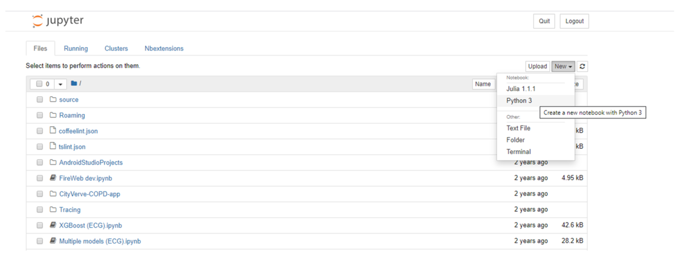
There are different ways of accessing Jupyter Notebooks. The Anaconda Distribution[8], a data science platform for Python and R, provides a free Python distribution, which includes Jupyter Notebooks. Another option includes JupyterHub[9], which is designed for groups of users to access notebooks on the cloud or locally hosted and maintained on their own devices. Once run, the user is greeted with a page showing the various files and folders available (Figure 5). Selecting the “new” option from the menu allows the user to create a new notebook in the selected language; alternatively, an existing notebook (ipynb) file can be loaded by selecting the required file from the list of files in the main list to the left of the screen.
|
Jupyter Notebooks, JupyterLab, and JupyterHub
Project Jupyter has created several resources and services surrounding the initial notebooks. This can sometimes cause some confusion among beginners. The difference among them are briefly described here.
- Jupyter Notebook is an interactive computational web application that combines code, text, data analysis, and other media in a single document.
- JupyterLab builds on the original Jupyter Notebook to provide an online interactive development environment that allows users to access notebooks with data and file viewers, text editors, and terminals all in the same environment. This helps to better integrate notebooks with other documents and resources in a single environment.
- JupyterHub allows multiple users (groups) to access notebooks and other resources. This can be useful for students and companies that want one or more groups to access and use a computational environment and resources without having to install and set things up. The management of these groups can be carried out by system administrators. Individual notebooks and the JupyterLab can be accessed via the Hub. The Hub can be run in the cloud or on a group's own hardware.
As these offerings build on the initial notebook and have notebooks at their core, this article describes the notebooks for beginners, rather than the additional platforms and services that incorporate them. Notebooks themselves work in a similar way regardless of being accessed alone or via JupyterLab or JupyterHub. It is worth being aware of these options, however, for building and sharing resources around the notebooks that you may develop.
Notebook extensions
A number of different “bolt on” extensions exists for the notebooks. These can be extremely useful for including additional features into a notebook. Some examples include the ability to split a cell into two different cells horizontally, a spellchecker, auto-numbering of equations, and an extension for making exercise tasks (discussed later). To enable and utilize the additional features that are available with the notebooks, the following commands should be entered into the command prompt (e.g., the Anaconda prompt or Powershell):
pip install jupyter_contrib_nbextensions
jupyter contrib nbextension install—user
pip install jupyter_nbextensions_configurator
jupyter nbextensions_configurator enable–user
This enables the “NBextensions” tab (Figure 6). When clicked on, the user is presented with a series of checkboxes for the various extensions. There is also a description, often with associated screenshots and/or animations previewing what the extension does.
|
When a new notebook is opened, the selected extensions appear as small icon buttons under the main menu (Figure 7).
|
Magic commands
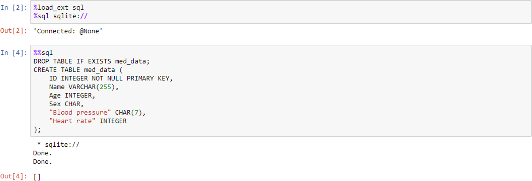
IPython (the “Interactive Python” kernel used in Jupyter Notebook) also supports what are known as magic commands or functions, which are used to change the standard behaviour of IPython. Magic commands come in two different types: “line” and “cell” magics. The %lsmagic command displays a list of all the available line magics, while %magic displays a help window with information about magic functions. A line magic only works on the line of code that it precedes, whereas a cell magic applies the function to the entire cell. A line magic is prefixed with a single percentage character (%), whereas a cell magic is prefixed with two percent characters (%%). Figure 8 shows an example of this, where we use the magic functions to load a Structured Query Language (SQL) extension and specify a database engine such as SQLite. The second code cell employs cell magic to allow us to write and execute SQL commands in the notebook environment to create a database table.
|
Widgets
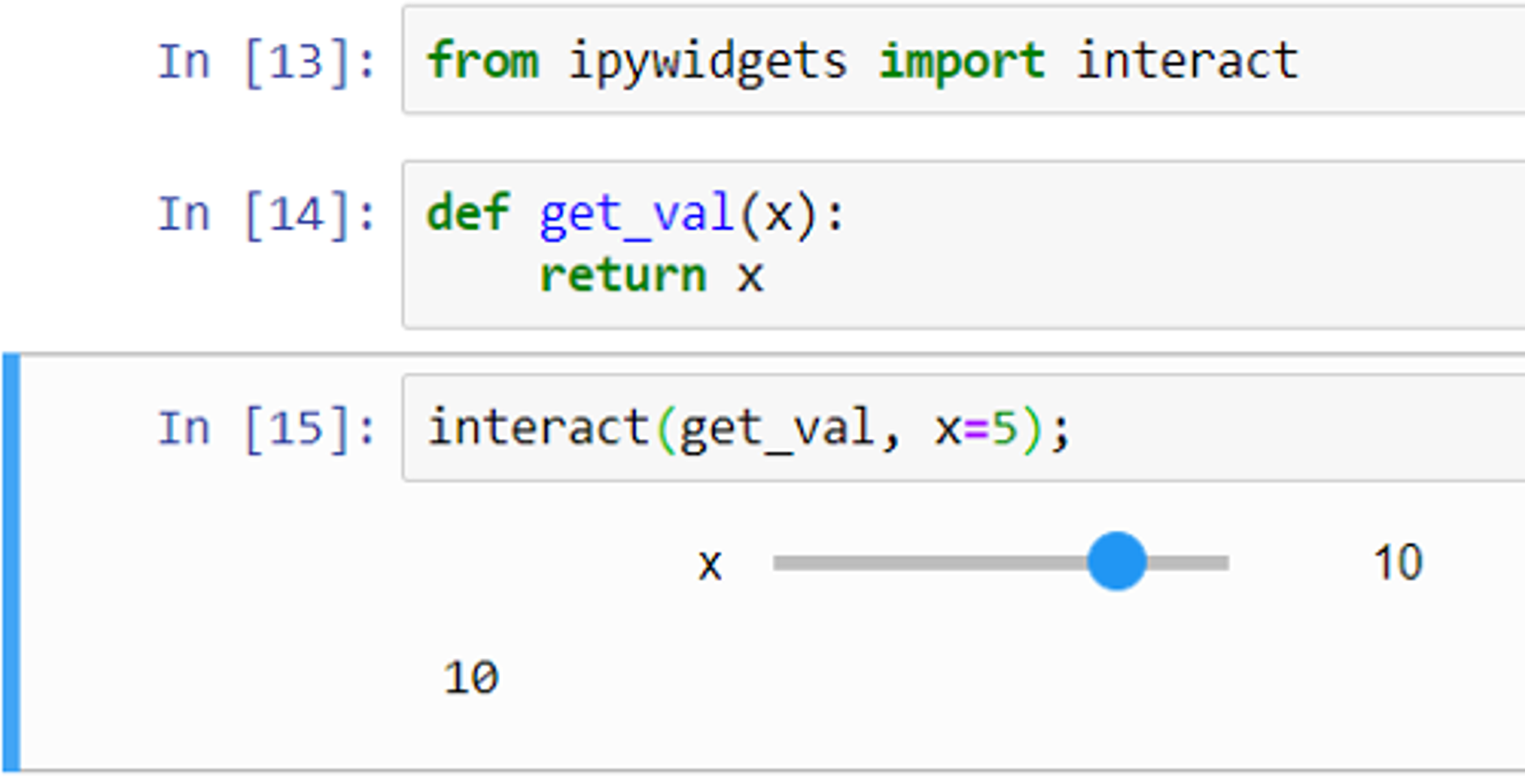
Widgets can be used for interactive elements in notebooks.[10] Figure 9 shows an example of this where the “interact” function runs the “get_val” function displaying a slider with the default value (5 in this case) selected. The user can then change the value by moving the slider to the left or right. Figure 10 shows another example, this time using a drop-down list of options created from a Python list.
|
|
A more substantive example of using interactive widgets is highlighted by Richardson and Behrang, who use Python notebooks to view Digital Imaging and Communications in Medicine (DICOM) images.[4]
How Jupyter enhances collaboration and reproducibility
Reproducibility in science is an important concept. Without reproducability, there is a lack of transparency about what was done. One would expect that if scientists follow the same method, the results will be the same. This is sometimes difficult to achieve with complex data and analysis methods. The quality of research in relation to collaboration was brought into question in a recent Wellcome Trust report on research culture that raised concerns over the impact of lack of research collaboration on research quality, and in some cases, unhealthy competition between researchers.[11] As Hardwicke and colleagues highlight, the availability of data is essential for a self-correcting ecosystem in science, which can be undermined by unclear analysis and poorly curated data, which, in turn, impedes analytic reproducibility.[12]
There has been a counter-movement to improve these issues by organizations such as the U.K. Reproducibility Network (UKRN)[13], which is a network of 10 universities in the U.K. that are concerned with reproducibility in research. The founder of UKRN calls for institutional changes to promote open-research practices.[14] Although various research studies do share their data, other researchers’ understanding of the shared dataset and their ability to repeat the previous analysis hinges on the documentation of both the dataset and analysis steps followed, as well as being able to replicate the software environment in order to run the code in the first instance. Because of these requirements, notebooks are being used increasingly by researchers to share analysis code along with an explanation and steps involved in processing the data for reproducible research purposes. This has led to widescale use in the research community.[15] By using interactive notebooks, the data analysis code and steps taken can be shared together with any additional documentation, formulas, etc. that are required to understand the applied method. Sharing data and analysis code in such a way dramatically improves the speed in which the analysis can be rerun by other researchers. Researches are also building on notebook technology for novel purposes, for example, Tellurium notebooks that were developed to support the creation of reproducible models for systems and synthetic biology.[16]
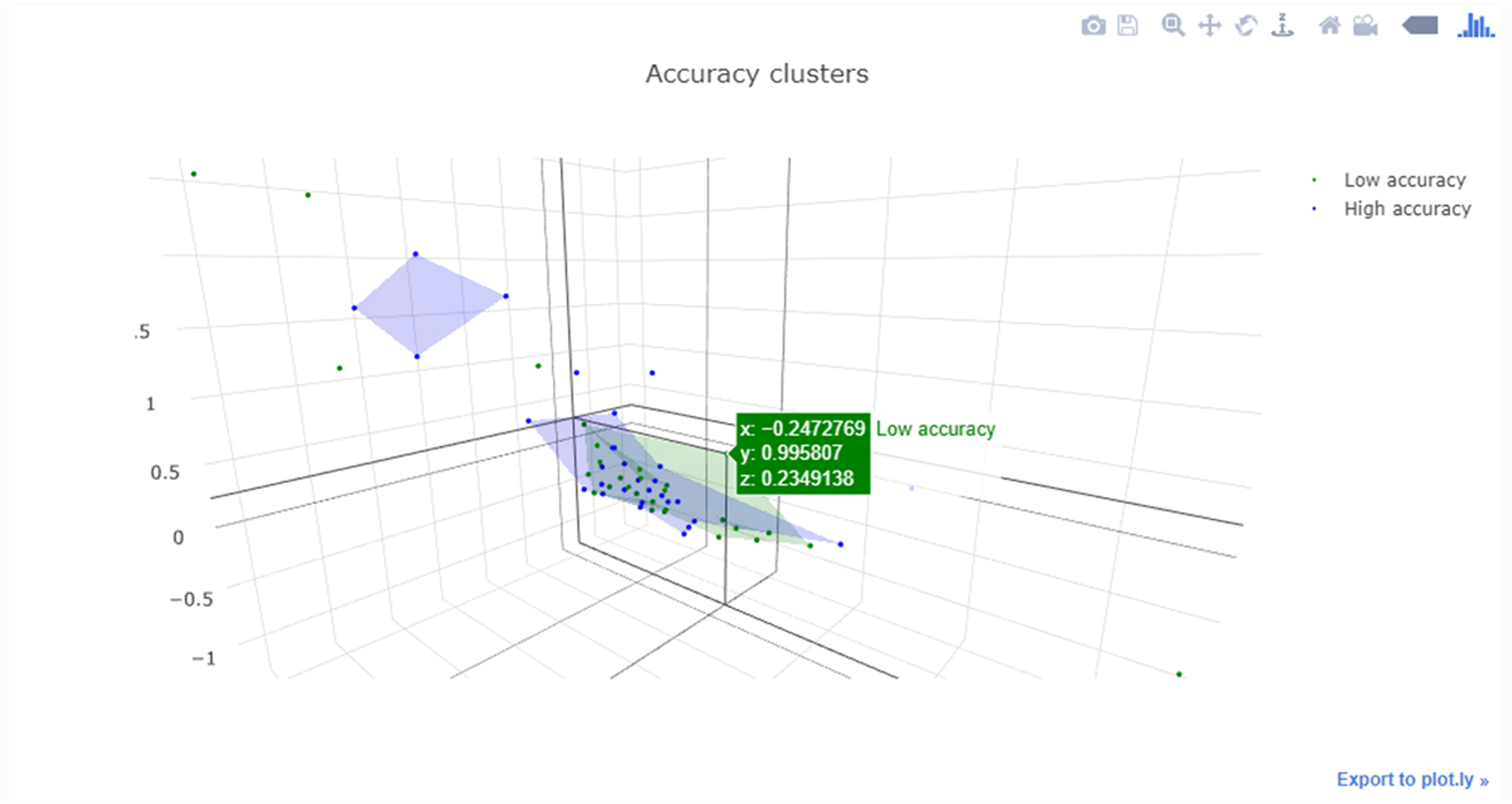
Aside from the research applications, Jupyter Notebooks are also being increasingly used to teach subjects like data science and programming[17], as they feature dynamic responses such as interactive visualizations and rapid updating of results based on the filtering of data (e.g., Figure 11).
|
Notebooks and assessment
Notebooks can also be set up to carry out formative or summative assessment. The “nbgrader” tool[18] allows for the creation and grading of assignments in the notebook environment. The tool allows a user to generate an instructor version of a notebook that has predefined solutions. This, in turn, is used to generate the student version of the notebooks without the solutions. These student versions of the notebook(s) can then be distributed to the students by email or via a virtual learning environment (VLE). The principal aims of the tool were to address issues surrounding the maintenance of separate student and instructor notebook versions, automatic grading of exercises, the manual grading of “free response” questions, and the ability to provide feedback to students. There are two ways of using the nbgrader. The first is a standalone version, while the second is designed to work with JupyterHub, which can manage the release and collection of submitted assessments. The nbgrader adds a tool bar to each cell to make the cell either an “answer” or a “test” cell. The answer cells allow students to add code placed between a placeholder. Unit tests are written by the instructor to evaluate the correctness of a student’s solution. Tests can also be hidden from the students. Points can be assigned to each cell to assign specified marks if the unit tests pass. Cells can also be set to “manually graded” answers so students can write free text, code formulas, etc. Student feedback can be provided when grading by adding text to any required cell and then converting the notebooks into HTML format so they can be emailed or added to VLE for the students to view.
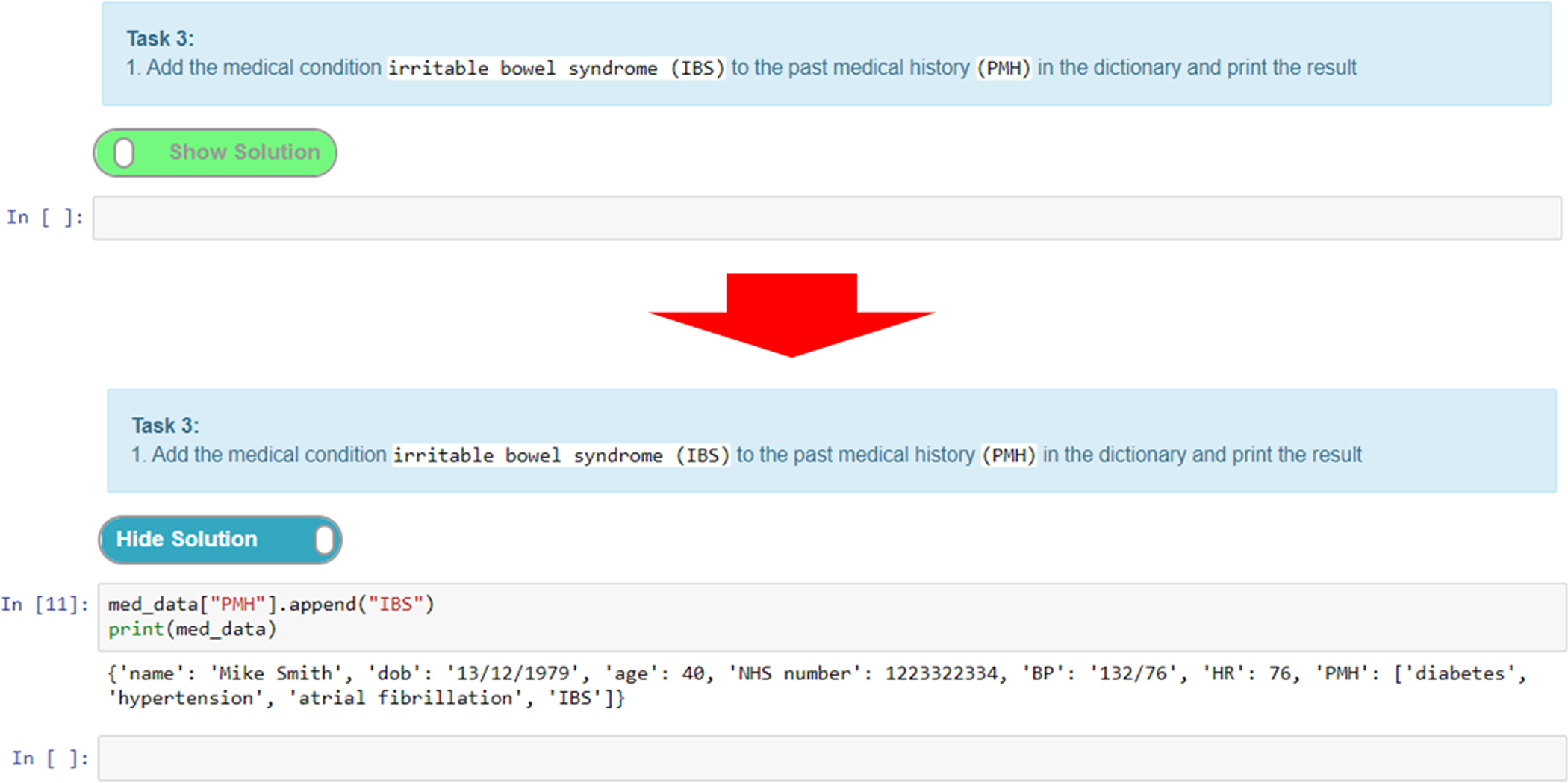
A simpler method of providing interactive tasks for formative assessment that does not require the knowledge of writing unit tests is to use the exercise extension. This extension can be used to add exercises (Figure 12). Adding feedback in the form of exercises is a unique feature of notebooks that elevates them from simply being an online textbook. The ability to provide interactive tasks that let students engage directly with the notebook without the need to use additional software is a powerful feature. Moreover, this helps maintain the narrative flow, as the exercises can be woven into the content in appropriate places without diverting the user to other tools or resources, all of which helps with the overall user experience.
|
Here, we give an example of an exercise where we create a task cell and put the solution in the preceding cell. The solution cell can be hidden until the “show solution” button (Figure 12) is activated, which reveals the hidden cell. This is a good way of adding coding tasks for students and then presenting them with a model answer or solution for comparison and/or further explanation. Figure 12 shows a task where the student has to add a textual value to a Python dictionary data structure and output the result. Students can attempt to write the code for this and then toggle the solution to check their answer with the one provided.
Sharing your notebooks
Notebooks can be shared in the same way as any other file. In order to run a notebook, however, users will need to install and set up software (i.e., Anaconda). This may not be the ideal solution given that novices may have difficulties installing and setting up the environment required to view and use notebooks. This is further compounded if the user needs to install extra libraries and extensions that may be required to run a notebook as intended. One helpful way around this when sharing notebooks with novices is the Binder project.[19]
Binder is a web service (currently open-source) that allows users to create interactive sharable and reproducible computational environments in the cloud.[20] Binder uses several different technologies (i.e., repo2docker, JupyterHub, and BinderHub) that allow a user to place their notebooks in a repository (e.g., GitHub). Once done, a form can be filled in on the Binder website (mybinder.org). This includes a repository Uniform Resource Locator (URL), Git tag, and optional path of the notebook file. Following this, a user will receive a URL that they can send to others to share their notebooks.
For a more technical explanation of how Binder works, please see the Binder paper presented at the SCIPY conference in 2018 and its associated YouTube video.[20] For more information on how to implement sharing Notebooks with Binder, see the Data Carpentry tutorial, which guides users through sharing their notebooks with GitHub and using Binder.[21]
References
- ↑ Gregory, J.; Salmon, G. (2013). "Professional development for online university teaching". Distance Education 34 (3): 256–70. doi:10.1080/01587919.2013.835771.
- ↑ Georgina, D.A.; Olson, M.R. (2008). "Integration of technology in higher education: A review of faculty self-perceptions". The Internet and Higher Education 11 (1): 1–8. doi:10.1016/j.iheduc.2007.11.002.
- ↑ 3.0 3.1 "Jupyter". Project Jupyter. https://jupyter.org/. Retrieved 27 January 2020.
- ↑ 4.0 4.1 Richardson, M.L.; Amini, B.. "Scientific Notebook Software: Applications for Academic Radiology". Current Problems in Diagnostic Radiology 47 (6): 368–77. doi:10.1067/j.cpradiol.2017.09.005. PMID 29122394.
- ↑ Cone, M.. "Markdown Guide". https://www.markdownguide.org/. Retrieved 23 September 2019.
- ↑ "An introduction to LaTeX". The LaTeX Project. https://www.latex-project.org/about/. Retrieved 27 January 2020.
- ↑ Roberts, A.; Oetiker, T.; Partl, H. et al.. "LaTeX/Mathematics". LaTeX - WikiBooks. https://en.wikibooks.org/wiki/LaTeX/Mathematics. Retrieved 27 January 2020.
- ↑ "Anaconda Distribution". Anaconda, Inc. 2019. Archived from the original on 06 September 2019. https://web.archive.org/web/20190906215334/https://www.anaconda.com/distribution/. Retrieved 21 September 2019.
- ↑ "JupyterHub". Project Jupyter. https://jupyter.org/hub. Retrieved 27 January 2020.
- ↑ "Using Interact". ipywidgets User Guide. Project Jupyter. https://ipywidgets.readthedocs.io/en/latest/examples/Using%20Interact.html.
- ↑ "What researchers think about the culture they work in". Wellcome Trust. 14 January 2020. https://wellcome.org/reports/what-researchers-think-about-research-culture.
- ↑ Hardwicke, T.E.; Mathur, M.B.; MacDonald, K. et al. (2018). "Data availability, reusability, and analytic reproducibility: Evaluating the impact of a mandatory open data policy at the journal Cognition". Royal Society Open Science 5 (8): 180448. doi:10.1098/rsos.180448.
- ↑ "U.K. Reproducibility Network". U.K. Reproducibility Network. https://www.ukrn.org/.
- ↑ Munafò, M. (2019). "Raising research quality will require collective action". Nature 576: 183. doi:10.1038/d41586-019-03750-7.
- ↑ Rule, A.; Birmingham, A.; Zuniga, C. et al. (2018). "Ten Simple Rules for Reproducible Research in Jupyter Notebooks". arXiv: 1–8. https://arxiv.org/abs/1810.08055.
- ↑ Medley, J.K.; Choi, K.; König, M. et al. (2018). "Tellurium notebooks—An environment for reproducible dynamical modeling in systems biology". PLOS Computational Biology 14 (6): e1006220. doi:10.1371/journal.pcbi.1006220.
- ↑ Barba, L.A.; Barker, L.J.; Blank, D.S. et al. (6 December 2019). "Teaching and Learning with Jupyter". GitHub. https://jupyter4edu.github.io/jupyter-edu-book/index.html. Retrieved 27 January 2020.
- ↑ "nbgrader". Jupyter Development Team. https://nbgrader.readthedocs.io/en/stable/. Retrieved 27 January 2020.
- ↑ "binder". Project Jupyter. https://mybinder.org/. Retrieved 05 June 2020.
- ↑ 20.0 20.1 Bussonnier, M.; Forde, J.; Freeman, J. et al. (2018). "Binder 2.0 - Reproducible, interactive, sharable environments for science at scale". Proceedings of the 17th Python in Science Conference: 113–20. doi:10.25080/Majora-4af1f417-011.
- ↑ Data Carpentry. "Sharing Jupyter Notebooks". GitHub. https://reproducible-science-curriculum.github.io/sharing-RR-Jupyter/. Retrieved 05 June 2020.
Notes
This presentation attempts to remain faithful to the original, with only a few minor changes to presentation. Grammar and punctuation has been updated reasonably to improve readability. In some cases important information was missing from the references, and that information was added. The original URL for the Anaconda Distribution is dead; an archived version of the URL was used for this version. The original "Using Interact" URL was also broken; an updated live version was substituted for this version. The UKRN URL also changed, and a current URL is used for this version.


